Fine-Tuning Vision Language Models (VLMs) for Data Extraction

Introduction

If you’re beginning your journey into the world of Vision Language Models (VLMs), you’re entering an exciting and rapidly evolving field that bridges the gap between visual and textual data. On the way to fully integrate VLMs into your business, there are roughly three phases you need to go through.

Choosing the Right Vision Language Model (VLM) for Your Business Needs

Selecting the right VLM for your specific use case is essential to unlocking its full potential and driving success for your business. A comprehensive survey of available models, can help you navigate the wide array of options, providing a solid foundation to understand their strengths and applications.

Identifying the Best VLM for Your Dataset

Once you’ve surveyed the landscape, the next challenge is identifying which VLM best suits your dataset and specific requirements. Whether you’re focused on structured data extraction, information retrieval, or another task, narrowing down the ideal model is key. If you’re still in this phase, this guide on selecting the right VLM for data extraction offers practical insights to help you make the best choice for your project.

Fine-Tuning Your Vision Language Model

Now that you’ve selected a VLM, the real work begins: fine-tuning. Fine-tuning your model is essential to achieving the best performance on your dataset. This process ensures that the VLM is not only capable of handling your specific data but also improves its generalization capabilities, ultimately leading to more accurate and reliable results. By customizing the model to your particular needs, you set the stage for success in your VLM-powered applications.

In this article, we will dive into the different types of fine-tuning techniques available for Vision Language Models (VLMs), exploring when and how to apply each approach based on your specific use case. We’ll walk through setting up the code for fine-tuning, providing a step-by-step guide to ensure you can seamlessly adapt your model to your data. Along the way, we will discuss important hyperparameters—such as learning rate, batch size, and weight decay—that can significantly impact the outcome of your fine-tuning process. Additionally, we will visualize the results of one such fine-tuning activity, comparing the old, pre-fine-tuned results from a previous post to the new, improved outputs after fine-tuning. Finally, we will wrap up with key takeaways and best practices to keep in mind throughout the fine-tuning process, ensuring you achieve the best possible performance from your VLM.

Types of Fine-Tuning

Fine-tuning is a critical process in machine learning, particularly in the context of transfer learning, where pre-trained models are adapted to new tasks. Two primary approaches to fine-tuning are LoRA (Low-Rank Adaptation) and Full Model Fine-Tuning. Understanding the strengths and limitations of each can help you make informed decisions tailored to your project’s needs.

LoRA (Low-Rank Adaptation)

LoRA is an innovative method designed to optimize the fine-tuning process. Here are some key features and benefits:

• Efficiency: LoRA focuses on modifying only a small number of parameters in specific layers of the model. This means you can achieve good performance without the need for massive computational resources, making it ideal for environments where resources are limited.

• Speed: Since LoRA fine-tunes fewer parameters, the training process is typically faster compared to full model fine-tuning. This allows for quicker iterations and experiments, especially useful in rapid prototyping phases.

• Parameter Efficiency: LoRA introduces low-rank updates, which helps in retaining the knowledge from the original model while adapting to new tasks. This balance ensures that the model does not forget previously learned information (a phenomenon known as catastrophic forgetting).

• Use Cases: LoRA is particularly effective in scenarios with limited labeled data or where the computational budget is constrained, such as in mobile applications or edge devices. It’s also beneficial for large language models (LLMs) and vision models in specialized domains.

Full Model Fine-Tuning

Full model fine-tuning involves adjusting the entire set of parameters of a pre-trained model. Here are the main aspects to consider:

• Resource Intensity: This approach requires significantly more computational power and memory, as it modifies all layers of the model. Depending on the size of the model and dataset, this can result in longer training times and the need for high-performance hardware.

• Potential for Better Results: By adjusting all parameters, full model fine-tuning can lead to improved performance, especially when you have a large, diverse dataset. This method allows the model to fully adapt to the specifics of your new task, potentially resulting in superior accuracy and robustness.

• Flexibility: Full model fine-tuning can be applied to a broader range of tasks and data types. It is often the go-to choice when there is ample labeled data available for training.

• Use Cases: Ideal for scenarios where accuracy is paramount and the available computational resources are sufficient, such as in large-scale enterprise applications or academic research with extensive datasets.

Prompt, Prefix and P Tuning

These three methods are used to identify the best prompts for your particular task. Basically, we add learnable prompt embeddings to an input prompt and update them based on the desired task loss. These techniques helps one to generate more optimized prompts for the task without training the model.

E.g., In prompt-tuning, for sentiment analysis the prompt can be adjusted from "Classify the sentiment of the following review:" to "[SOFT-PROMPT-1] Classify the sentiment of the following review: [SOFT-PROMPT-2]" where the soft-prompts are embeddings which don't have any real world significance but will give a stronger signal to the LLM that user is looking for sentiment classification, removing any ambiguity in the input. Prefix and P-Tuning are somewhat variations on the same concept where Prefix tuning interacts more deeply with the model’s hidden states because it is processed by the model’s layers and P-Tuning uses more continuous representations for tokens

Quantization-Aware Training

This is an orthogonal concept where either full-finetuning or adapter-finetuning occur in lower precision, reducing memory and compute. QLoRA is one such example.

Mixture of Experts (MoE) Fine-tuning

Mixture of Experts (MoE) fine-tuning involves activating a subset of model parameters (or experts) for each input, allowing for efficient resource usage and improved performance on specific tasks. In MoE architectures, only a few experts are trained and activated for a given task, leading to a lightweight model that can scale while maintaining high accuracy. This approach enables the model to adaptively leverage specialized capabilities of different experts, enhancing its ability to generalize across various tasks while reducing computational costs.

Considerations for Choosing a Fine-Tuning Approach

When deciding between LoRA and full model fine-tuning, consider the following factors:

• Computational Resources: Assess the hardware you have available. If you are limited in memory or processing power, LoRA may be the better choice.
• Data Availability: If you have a small dataset, LoRA’s efficiency might help you avoid overfitting. Conversely, if you have a large, rich dataset, full model fine-tuning could exploit that data fully.
• Project Goals: Define what you aim to achieve. If rapid iteration and deployment are crucial, LoRA’s speed and efficiency may be beneficial. If achieving the highest possible performance is your primary goal, consider full model fine-tuning.
• Domain Specificity: In specialized domains where the nuances are critical, full model fine-tuning may provide the depth of adjustment necessary to capture those subtleties.
• Overfitting: It is important to keep an eye on validation loss to ensure that the we are not over learning on the training data
• Catastrophic Forgetting: This refers to the phenomenon where a neural network forgets previously learned information upon being trained on new data, leading to a decline in performance on earlier tasks. This is also called as Bias Amplification or Over Specialization based on context. Although similar to overfitting, catastrophic forgetting can occur even when a model performs well on the current validation dataset.

To Summarize -

Prompt tuning, LoRA and full model fine-tuning have their unique advantages and are suited to different scenarios. Understanding the requirements of your project and the resources at your disposal will guide you in selecting the most appropriate fine-tuning strategy. Ultimately, the choice should align with your goals, whether that’s achieving efficiency in training or maximizing the model’s performance for your specific task.

As per the previous article, we have seen that Qwen2 model has given the best accuracies during data extraction. Continuing the flow, in the next section, we are going to fine-tune Qwen2 model on CORD dataset using LoRA finetuning.

Setting Up for Fine-Tuning

Step 1: Download LLama-Factory

To streamline the fine-tuning process, you’ll need LLama-Factory. This tool is designed for efficient training of VLMs.

git clone https://github.com/hiyouga/LLaMA-Factory/ /home/paperspace/LLaMA-Factory/

Step 2: Create the Dataset

Format your dataset correctly. A good example of dataset formatting comes from ShareGPT, which provides a ready-to-use template. Make sure your data is in a similar format so that it can be processed correctly by the VLM.

ShareGPT's format deviates from huggingface format by having the entire ground truth present inside a single JSON file -

[
    {
        "messages": [
            {
                "content": "<QUESTION>\n<image>",
                "role": "user"
            },
            {
                "content": "<ANSWER>",
                "role": "assistant"
            }
        ],
        "images": [
            "/home/paperspace/Data/cord-images//0.jpeg"
        ]
    },
    ...
    ...
]

Creating the dataset in this format is just a question of iterating the huggingface dataset and consolidating all the ground truths into one json like so -

# https://github.com/NanoNets/hands-on-vision-language-models/blob/main/src/vlm/data/cord.py

cli = Typer()

prompt = """Extract the following data from given image - 

For tables I need a json of list of 
dictionaries of following keys per dict (one dict per line)
'nm', # name of the item
'price', # total price of all the items combined
'cnt', # quantity of the item
'unitprice' # price of a single igem

For sub-total I need a single json of
{'subtotal_price', 'tax_price'}

For total I need a single json of
{'total_price', 'cashprice', 'changeprice'}

the final output should look like and must be JSON parsable
{
    "menu": [
        {"nm": ..., "price": ..., "cnt": ..., "unitprice": ...}
        ...
    ],
    "subtotal": {"subtotal_price": ..., "tax_price": ...},
    "total": {"total_price": ..., "cashprice": ..., "changeprice": ...}
}
If a field is missing,
simply omit the key from the dictionary. Do not infer.
Return only those values that are present in the image.
this applies to highlevel keys as well, i.e., menu, subtotal and total
"""


def load_cord(split="test"):
    ds = load_dataset("naver-clova-ix/cord-v2", split=split)
    return ds

def make_message(im, item):
    content = json.dumps(load_gt(item).d)
    message = {
        "messages": [
            {"content": f"{prompt}<image>", "role": "user"},
            {"content": content, "role": "assistant"},
        ],
        "images": [im],
    }
    return message


@cli.command()
def save_cord_dataset_in_sharegpt_format(save_to: P):
    save_to = P(save_to)
    cord = load_cord(split="train")
    messages = []
    makedir(save_to)
    image_root = f"{parent(save_to)}/images/"
    for ix, item in E(track2(cord)):
        im = item["image"]
        to = f"{image_root}/{ix}.jpeg"
        if not exists(to):
            makedir(parent(to))
            im.save(to)
        message = make_message(to, item)
        messages.append(message)
    return write_json(messages, save_to / "data.json")

Once the cli command is in place - You can create the dataset anywhere on your disk.

vlm save-cord-dataset-in-sharegpt-format /home/paperspace/Data/cord/

Step 3: Register the Dataset

Llama-Factory needs to know where the dataset exists on the disk along with the dataset format and the names of keys in the json. For this we have to modify the data/dataset_info.json json file in the Llama-Factory repo, like so -

from torch_snippets import read_json, write_json

dataset_info = '/home/paperspace/LLaMA-Factory/data/dataset_info.json'
js = read_json(dataset_info)
js['cord'] = {
    "file_name": "/home/paperspace/Data/cord/data.json",
    "formatting": "sharegpt",
    "columns": {
      "messages": "messages",
      "images": "images"
    },
    "tags": {
      "role_tag": "role",
      "content_tag": "content",
      "user_tag": "user",
      "assistant_tag": "assistant"
    }
  }
write_json(js, dataset_info)

Step 4: Set Hyperparameters

Hyperparameters are the settings that will govern how your model learns. Typical hyperparameters include the learning rate, batch size, and number of epochs. These may require fine-tuning themselves as the model trains.

### model
model_name_or_path: Qwen/Qwen2-VL-2B-Instruct

### method
stage: sft
do_train: true
finetuning_type: lora
lora_target: all

### dataset
dataset: cord
template: qwen2_vl
cutoff_len: 1024
max_samples: 1000
overwrite_cache: true
preprocessing_num_workers: 16

### output
output_dir: saves/cord-4/qwen2_vl-2b/lora/sft
logging_steps: 10
save_steps: 500
plot_loss: true
overwrite_output_dir: true

### train
per_device_train_batch_size: 8
gradient_accumulation_steps: 8
learning_rate: 1.0e-4
num_train_epochs: 10.0
lr_scheduler_type: cosine
warmup_ratio: 0.1
bf16: true
ddp_timeout: 180000000

### eval
val_size: 0.1
per_device_eval_batch_size: 1
eval_strategy: steps
eval_steps: 500

We begin by specifying the base model, Qwen/Qwen2-VL-2B-Instruct. As mentioned above, we are using Qwen2 as our starting point depicted by the variable model_name_or_path

Our method involves fine-tuning with LoRA (Low-Rank Adaptation), focusing on all layers of the model. LoRA is an efficient finetuning strategy, allowing us to train with fewer resources while maintaining model performance. This approach is particularly useful for our structured data extraction task using the CORD dataset.

Cutoff length is used to limit the transformer's context length. Datasets where examples have very large questions/answers (or both) need a larger cutoff length and in turn need a larger GPU VRAM. In the case of CORD the max length of question and answers is not more than 1024 so we use it to filter any anomalies that might be present in one or two examples.

We're leveraging 16 preprocessing workers to optimize data handling. The cache is overwritten each time for consistency across runs.

Training details are also optimized for performance. A batch size of 8 per device, combined with gradient accumulation steps set to 8, allows us to effectively simulate a larger batch size of 64 examples per batch. The learning rate of 1e-4 and cosine learning rate scheduler with a warmup ratio of 0.1 help the model gradually adjust during training.

10 is a good starting point for the number of epochs since our dataset has only 800 examples. Usually, we aim for anything between 10,000 to 100,000 total training samples based on the variations in the image. As per above configuration, we are going with 10x800 training samples. If the dataset is too large and we need to train only on a fraction of it, we can either reduce the num_train_epochs to a fraction or reduce the max_samples to a smaller number.

Evaluation is integrated into the workflow with a 10% validation split, evaluated every 500 steps to monitor progress. This strategy ensures that we can track performance during training and adjust parameters if necessary.

Step 5: Train the Adapter Model

Once everything is set up, it’s time to start the training process. Since we’re focusing on fine-tuning, we’ll be using an adapter model, which integrates with the existing VLM and allows for specific layer updates without retraining the entire model from scratch.

llamafactory-cli train examples/train_lora/cord.yaml

Training for 10 epochs used approximately 20GB of GPU VRAM and ran for about 30 minutes.

Evaluating the Model

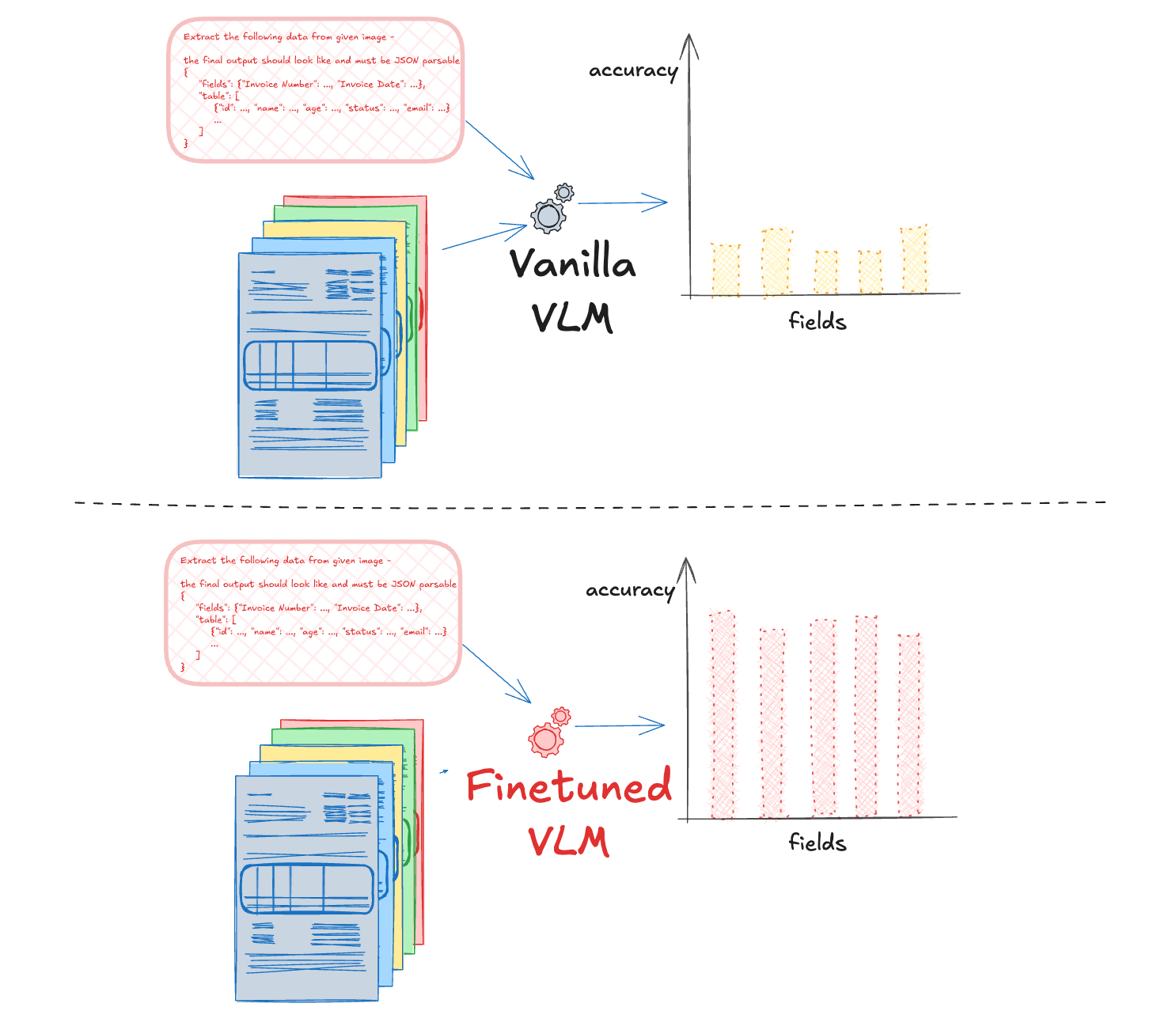
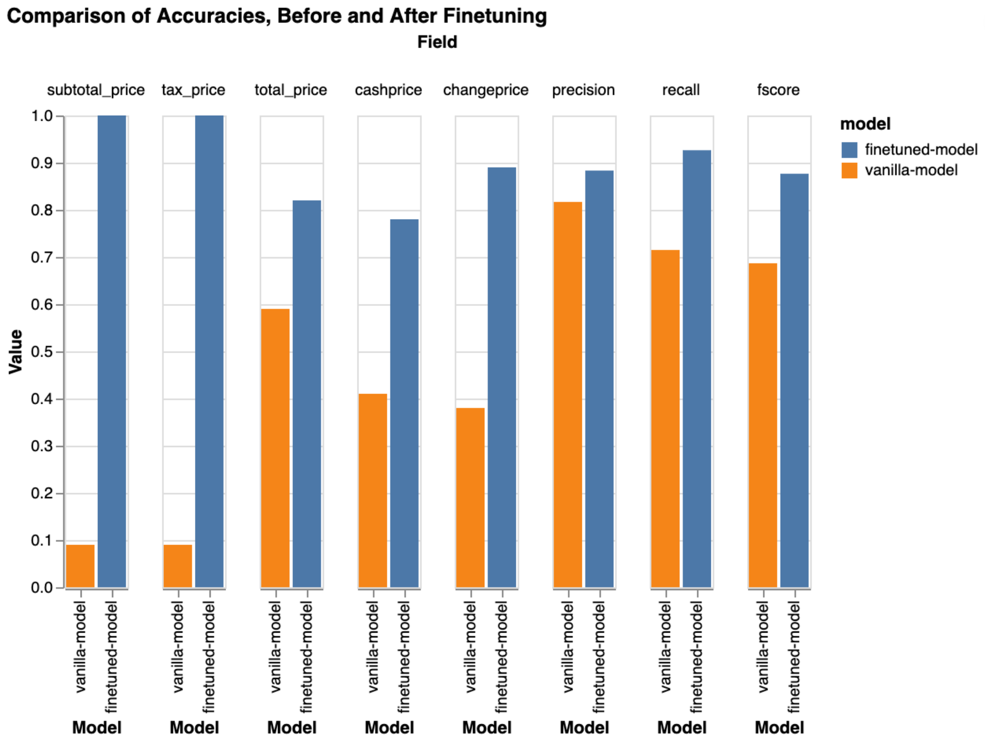
Once the model has been fine-tuned, the next step is to run predictions on your dataset to evaluate how well it has adapted. We will compare the previous results under the group vanilla-model and the latest outcomes under the group finetuned-model.

As shown below, there is a considerable improvement in many key metrics, demonstrating that the new adapter has successfully adjusted to the dataset.

Things to Keep in Mind

• Multiple Hyperparameter Sets: Fine-tuning isn't a one-size-fits-all process. You'll likely need to experiment with different hyperparameter configurations to find the optimal setup for your dataset.
• Training full model or LoRA: If training with an adapter shows no significant improvement, it’s logical to switch to full model training by unfreezing all parameters. This provides greater flexibility, increasing the likelihood of learning effectively from the dataset.
• Thorough Testing: Be sure to rigorously test your model at every stage. This includes using validation sets and cross-validation techniques to ensure that your model generalizes well to new data.
• Filtering Bad Predictions: Mistakes in your newly fine-tuned model can reveal underlying issues in the predictions. Use these mistakes to filter out bad predictions and refine your model further.
• Data/Image augmentations: Utilize image augmentations to expand your dataset, enhancing generalization and improving fine-tuning performance.

Conclusion

Fine-tuning a VLM can be a powerful way to enhance your model’s performance on specific datasets. By carefully selecting your tuning method, setting the right hyperparameters, and thoroughly testing your model, you can significantly improve its accuracy and reliability.