Introduction
While I do not like getting pulled over by cops any more than you do, I can't deny that having cameras that can track and count the vehicles passing by attached to traffic lights might just do some good for society.
Computers are getting better everyday at thinking, analyzing situations and making decisions like humans do. Understanding vision is an integral part of this progress in the area of machine intelligence. One of the things that has baffled scientists and engineers is how to get our algorithms to see things not pixel to pixel but capture the overarching patterns in a picture or a video. Object detection and object tracking technology have come far in that regard and the boundaries are being challenged and pushed as we talk.
While detecting objects in an image has been getting a lot of attention from the scientific community, a lesser known and yet an area with widespread applications is tracking objects in a video, something that requires us to merge our knowledge of detecting objects in static images with analysing temporal information and using it to best predict trajectories. Think tracking sports events, catching burglars, automating speeding tickets or if your life is a little more miserable, alert yourself when your three year old kid runs out the door without assistance.
Single object tracking
Probably the most cracked and the easiest of the tracking sub-problems is the single object tracking. In this, the objective is to simply lock onto a single object in the image and track it until it exits the frame. This type of tracking is relatively easier as the bigger problem of distinguishing this object from others doesn’t necessarily arise.
Multiple object tracking
In this type of tracking, we are expected to lock onto every single object in the frame, uniquely identify each one of them and track all of them until they leave the frame.
Object detection vs Object Tracking
These days, with the jargon surrounding deep learning, terms and their meanings tend to get mixed up, causing immense confusion to a new learner. So, what’s the difference between “Object Detection” and “Object Tracking”?
In object detection, we detect an object in a frame, put a bounding box or a mask around it, and classify the object. Note that the job of the detector ends here. It processes each frame independently and identifies numerous objects in that particular frame.
Now, an object tracker, on the other hand, needs to track a particular object across the entire video. If the detector detects 3 cars in the frame, the object tracker has to identify the 3 separate detections and track them across subsequent frames (with the help of a unique ID).
For this, the tracker needs to use spatio-temporal features. Techniques such as Raspberry Pi object detection can also be employed for real-time or edge computing scenarios. We shall look into this in later sections.
Challenges
Tracking an object on a straight road or a clear area might sound very easy. But hardly any real world application is that straight forward and free of any challenges. Here are some common problems one might encounter while using an object tracker.
Occlusion
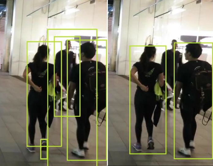
Occlusion of objects in videos is one of the most common obstacles to seamless tracking of objects. As you can see, in top figure (left), the man in the background is detected, while the same guy goes undetected in the next frame (right). Now, the challenge for the tracker lies in identifying the same guy when he is detected in a much later frame and associating his older track and features with his trajectory.
Variations in view points
Often in tracking, the objective will be to track an object across different cameras. As a consequence of this, there will be significant changes in how we view the object. This is illustrated in figure 3. In such cases the features used to track an object become very important as we need to make sure they are invariant to the changes in views. Later when we code our own tracker, we shall see how to effectively overcome this.
Non stationary camera
When the camera used for tracking a particular object is also in motion with respect to the object, it can often lead to unintended consequences. As I mentioned previously, many trackers consider the features from an object to track them. Such tracker might fail in scenarios where the object appears different because of the camera motion (appear bigger or smaller). A robust tracker for this problem can be very helpful in important applications like object tracking drones, autonomous navigation.
Annotating training data
One of the most annoying things about building an object tracker is getting good training data for a particular scenario. Unlike building a dataset for an object detector, where randomly unconnected images where the object is seen can be annotated, we require video sequences where each instance of the object is identified throughout, for each frame.
Traditional Methods
Meanshift
Meanshift or Mode seeking is a popular algorithm, which is mainly used in clustering and other related unsupervised problems. It is similar to K-Means, but replaces the simple centroid technique of calculating the cluster centers with a weighted average that gives importance to points that are closer to the mean. The goal of the algorithm is to find all the modes in the given data distribution. Also, this algorithm does not require an optimum “K” value like K-Means. More info on this can be found here.
Suppose we have a detection for an object in the frame and we extract certain features from the detection (colour, texture, histogram etc). By applying the meanshift algorithm, we have a general idea of where the mode of the distribution of features lies in the current state. Now when we have the next frame, where this distribution has changed due to the movement of the object in the frame, the meanshift algo looks for the new largest mode and hence tracks the object.
Optical flow
This method differs from the above two methods, as we do not necessarily use features extracted from the detected object. Instead, the object is tracked using the spatio-temporal image brightness variations at a pixel level.
Here we focus on obtaining a displacement vector for the object to be tracked across the frames. Tracking with optical flow rests on three important assumptions:
- Brightness consistency: Brightness around a small region is assumed to remain nearly constant, although the location of the region might change.
- Spatial coherence: Neighboring points in the scene typically belong to the same surface and hence typically have similar motions
- Temporal persistence: Motion of a patch has a gradual change.
- Limited motion: Points do not move very far or in a haphazard manner.
Once these criteria are satisfied, we use something called the Lucas-Kanade method to obtain an equation for the velocity of certain points to be tracked (usually these are easily detected features). Using the equation and some prediction techniques, a given object can be tracked throughout the video.
Kalman Filters
In almost any engineering problem that involves prediction in a temporal or time series sense, be it computer vision, guidance, navigation or even economics, “Kalman Filter” is the go to algorithm.
Core idea
The core idea of a Kalman filter is to use the available detections and previous predictions to arrive at a best guess of the current state, while keeping the possibility of errors in the process.
In our case, assume we have a fairly good enough object detector that detects car. But it is not that accurate also, and occasionally misses detections, say 1 in 10 frames. To effectively track and predict the next state of the car, let us assume a “Constant velocity model”. Now, once we have defined the simple model according to laws of physics, given a current detection, we can make a nice guess on where the car will be in the next frame. It all sounds perfect, in an ideal world. But, as I said before, there is always a noise component. So we have:
- Noise associated with the constant velocity model that we assumed cars would follow. It is obvious as we cannot expect a constant velocity always. We call this “Process Noise”.
- Since, the detector output, based on which we are making predictions is also not accurate, we have “Measurement Noise” associated with it.
As we see in the above pic, the Kalman filter works recursively, where we take current readings, to predict the current state, then use the measurements and update our predictions. So, it essentially boils down to inferring a new distribution (the predictions) from the previous state distribution and the measurement distribution.
The complete mathematical formulation and derivations with respect to the kalman filter are beyond the scope of this blog. However, it is recommended for you to go through them. You can follow these links to learn more: video; notes.
Why kalman works
Kalman filter works best for linear systems with Gaussian processes involved. In our case the tracks hardly leave the linear realm and also, most processes and even noise in fall into the Gaussian realm. So, the problem is suited for the use of Kalman filters.
Deep Learning based Approaches
Deep Regression Networks (ECCV, 2016) Paper: click here
One of the early methods that used deep learning, for single object tracking. A model is trained on a dataset consisting of videos with labelled target frames. The objective of the model is to simply track a given object from the given image crop.
To achieve this, they use a two-frame CNN architecture which uses both the current and the previous frame to accurately regress on to the object.
As shown in the figure, we take the crop from the previous frame based on the
predictions and define a “Search region” in the current frame based on that crop. Now the network is trained to regress for the object in this search region
The network architecture is simple with CNN’s followed by Fully connected layers that directly give us the bounding box coordinates.
ROLO - Recurrent Yolo (ISCAS 2016) click here
An elegant method to track objects using deep learning. Slight modifications to YOLO detector and attaching a recurrent LSTM unit at the end, helps in tracking objects by capturing the spatio-temporal features.
As shown above, the architecture is quite simple. The Detections from YOLO (bounding boxes) are concatenated with the feature vector from a CNN based feature extractor (We can either re-use the YOLO backend or use a specialised feature extractor). Now, this concatenated feature vector, which represents most of the spatial information related to the current object, along with the information on previous state is passed onto the LSTM cell.
The output of the cell, now accounts for both spatial and temporal information. This simple trick of using CNN’s for feature extraction and LSTM’s for bounding box predictions gave high improvements to tracking challenges.
Deep SORT (Deep Simple Online Real-Time Tracking)
Deep SORT (Deep Simple Online Real-Time Tracking) is a powerful tracking algorithm. It seamlessly combines deep learning for spotting objects with a tracking algorithm. This mix ensures precise and robust tracking, especially in busy and complex environments.
Deep SORT is one of the most popular and most widely used, elegant object tracking framework, It is an extension to SORT (Simple Real time Tracker). We shall go through the concepts introduced in brief and delve into the implementation. Let us take a close look at the moving parts in this paper.
The Kalman filter
Our friend from above, Kalman filter is a crucial component in deep SORT. Our state contains 8 variables; (u,v,a,h,u’,v’,a’,h’) where (u,v) are centres of the bounding boxes, a is the aspect ratio and h, the height of the image. The other variables are the respective velocities of the variables.
As we discussed previously, the variables have only absolute position and velocity factors, since we are assuming a simple linear velocity model. The Kalman filter helps us factor in the noise in detection and uses prior state in predicting a good fit for bounding boxes.
For each detection, we create a “Track”, that has all the necessary state information. It also has a parameter to track and delete tracks that had their last successful detection long back, as those objects would have left the scene.
Also, to eliminate duplicate tracks, there is a minimum number of detections threshold for the first few frames.
The assignment problem
Now that we have the new bounding boxes tracked from the Kalman filter, the next problem lies in associating new detections with the new predictions. Since they are processed independently, we have no idea on how to associate track_i with incoming detection_k.
To solve this, we need 2 things: A distance metric to quantify the association and an efficient algorithm to associate the data.
The distance metric
The authors decided to use the squared Mahalanobis distance (effective metric when dealing with distributions) to incorporate the uncertainties from the Kalman filter. Thresholding this distance can give us a very good idea on the actual associations. This metric is more accurate than say, euclidean distance as we are effectively measuring distance between 2 distributions (remember that everything is distribution under Kalman!)
The efficient algorithm
In this case, we use the standard Hungarian algorithm, which is very effective and a simple data association problem. I won’t delve into it’s details. More on this can be found here.
Lucky for us, it is a single line import on sklearn !
Where is deep learning in all this?
Well, we have an object detector giving us detections, Kalman filter tracking it and giving us missing tracks, the Hungarian algorithm solving the association problem. So, is deep learning really needed here ?
The answer is Yes. Despite the effectiveness of Kalman filter, it fails in many of the real world scenarios we mentioned above, like occlusions, different view points etc.
So, to improve this, the authors of Deep sort introduced another distance metric based on the “appearance” of the object.
The appearance feature vector
The idea to obtain a vector that can describe all the features of a given image is quite simple. We first build a classifier over our dataset, train it till it achieves a reasonably good accuracy, and then strip the final classification layer. Assuming a classical architecture, we will be left with a dense layer producing a single feature vector, waiting to be classified.
That feature vector becomes our “appearance descriptor” of the object.
The “Dense 10” layer shown in the above pic will be our appearance feature vector for the given crop. Once trained, we just need to pass all the crops of the detected bounding box from the image to this network and obtain the “128 X 1” dimensional feature vector.
Now, the updated distance metric will be :
\\(D = \lambda \cdot D_k + (1 - \lambda) \cdot D_a\\)
Where:
- \\(D_k\\): The Mahalanobis distance.
- \\(D_a\\): The cosine distance between appearance feature vectors.
- \\(\lambda\\): The weighting factor.
Interestingly, the importance of \\(D_a\\) is so significant that the authors claim state-of-the-art performance could be achieved even with \\(\lambda = 0\\)—i.e., relying solely on \\(D_a\\)!
This demonstrates how a simple distance metric, paired with a robust deep learning model, makes Deep SORT an elegant and widely used object tracker.
Code Review
In this section, we shall implement our own generic object tracker on a vehicle dataset.
Clone this repo and follow the setup instructions from README.md
Now, since we are interested in creating an object tracker and not a detector, we shall use a video with pre-existing detection outputs. The repo has a video with detection boxes from YOLO, SSD and Mask-RCNN.
The deep_sort folder in the repo has the original deep sort implementation, complete with the Kalman filter, hungarian algorithm and feature extractor. But the original repo is built only for validating the algorithm with the MARS test dataset. So, we have written a custom class deepsort.py that acts as a bridge and also takes in any custom configurations like a different feature extractor and other parameters.
Let us look at deepsort.py in detail.
class deepsort_rbc():
	def __init__(self):
		#loading this encoder is slow, should be done only once.
		self.encoder = torch.load('model640.pt')
		self.encoder = self.encoder.cuda()
		self.encoder = self.encoder.eval()
		print("Deep sort model loaded")

		self.metric = nn_matching.NearestNeighborDistanceMetric("cosine",.5 , 100)
		self.tracker= Tracker(self.metric)

		self.gaussian_mask = get_gaussian_mask().cuda()
The self.encoder variable of the class loads the feature extractor once an object of this class is created. We need to make sure that we load this instance only once, for a run.
The self.metric variable defines the distance metric to be used in the Hungarian algorithm for the data association problem.
self.tracker is an object of the class Tracker defined in the deep_sort library, that takes care of creation, keeping track and eventual deletion of all tracks.
self.gaussian_mask is our not so important creation, that we shall talk about in the next section.
run_deep_sort is the main function of this class, that we would be using. It takes in the frame, the detected bounding boxes and their confidence scores and returns an instance of the Tracker class that has all the info pertaining to the current tracks.
An overview of the program flow:
#Initialize deep sort object.
deepsort = deepsort_rbc(wt_path='ckpts/model640.pt') #path to the feature extractor model.

#Obtain all the detections for the given frame.
detections,out_scores = get_gt(frame,frame_id,gt_dict)

#Pass detections to the deepsort object and obtain the track information.
tracker,detections_class = deepsort.run_deep_sort(frame,out_scores,detections)

#Obtain info from the tracks.
for track in tracker.tracks:
    bbox = track.to_tlbr() #Get the corrected/predicted bounding box
    id_num = str(track.track_id) #Get the ID for the particular track.
    features = track.features #Get the feature vector corresponding to the detection.
We can look into test_on_video.py file to see a similar flow, where we test the deep_sort framework on the given video.
The pre_process function is used to convert the cropped detection images into an input as expected by the feature extractor network. In our case that would be just resizing them to 128X128 and converting to a torch tensor.
Training your own feature extractor
Since, the original deepsort focused on MARS dataset, which is based on people, the feature extractor is trained on humans. We need an equivalent feature extractor for vehicles. We shall be training a Siamese network for the same. More info on siamese nets can be found here and here.
We shall be using a Siamese network with a triplet loss function for our task. Siamese nets are known to work great for feature matching problems as they are trained to keep together data points of similar features and at the same time, learn to keep the entire group far away from other such groups. This is exactly what we need, as we want the same ID for a vehicle in different views and different IDs for different vehicles.
So, to achieve this desired result, during training, we take 3 images -> the anchor (which is the training image), a positive (another image from the same class as the anchor), and a negative (another image from any other class). The objective of the loss function of the CNN network would be to minimize the cosine distance between feature vectors of anchor and the positive image and also simultaneously maximize the cosine distance between feature vectors of anchor and the negative image. The loss is illustrated below (Note that 1 is similar and 0 is dissimilar in cosine metric)
        distance_positive = F.cosine_similarity(anchor,positive)
        distance_negative = F.cosine_similarity(anchor,negative)
        loss = (1- distance_positive)**2 + (0 - distance_negative)**2
We have a training and testing set, extracted from the NVIDIA AI city Challenge dataset. You can download it from here.
Extract the crops/ and crops_test/ folders in the same working directory. Both folders have 184 different sub-folders, each of which contains crops of a certain vehicle, shot in various views.We need to maintain a similar folder structure to train for any other custom dataset. Once, the folders have been extracted, we can go through the network configurations and the various options in siamese_net.py and siamese_dataloader.py
siamese_net.py has the network configuration. The net consists entirely of CNN layers with ReLU activation and batch normalization. It also has the definitions for both contrastive and triplet loss functions.
siamese_dataloader.py has the definitions for the unique data loader we would be requiring for our task. It has functions to randomly select the anchor, positive and negative images and also apply any required data augmentations.
siamese_train.py has the code to train our network. Since we are dealing with cropped outputs from an object detector, the boxes might not be a perfect fit; Hence,there is a possibility of background elements influencing the values of the feature vector. In order to avoid that, we multiply the input training image with a 2D-Gaussian mask.This will act like a visual attention mechanism, by forcing the network to focus more on the center of the cropped image and give less importance to the background elements. The get_gaussian_mask function takes care of this.
Since, we have trained our network with a gaussian mask, it only makes sense to continue to use the same during inference as well. So, we have the self.gaussian_mask variable in deepsort.py which is used during inference.
siamese_test.py lets us know the accuracy of the trained feature vector by randomly sampling images and comparing them with distances from negatives and positives.
Now that our own feature extractor is trained and tested, we are ready to launch our custom object tracker! Just follow the stub code given in test_on_video.py to build your own program flows.
Conclusion
I hope this blog has helped you gain a comprehensive understanding of the core ideas and components in object tracking and acquainted you with the tools required to build your own custom object detector. Get coding and make sure there are no strays in your front yard anymore ever!
Lazy to code, don't want to spend on GPUs? Head over to Nanonets and build computer vision models for free!