How to do Semantic Segmentation using Deep learning
This article is a comprehensive overview including a step-by-step guide to implement a deep learning image segmentation model.
We shared a new updated blog on Semantic Segmentation here: A 2021 guide to Semantic Segmentation
Nowadays, semantic segmentation is one of the key problems in the field of computer vision. Looking at the big picture, semantic segmentation is one of the high-level task that paves the way towards complete scene understanding. The importance of scene understanding as a core computer vision problem is highlighted by the fact that an increasing number of applications nourish from inferring knowledge from imagery. Some of those applications include self-driving vehicles, human-computer interaction, virtual reality etc. With the popularity of deep learning in recent years, many semantic segmentation problems are being tackled using deep architectures, most often Convolutional Neural Nets, which surpass other approaches by a large margin in terms of accuracy and efficiency.
What is Semantic Segmentation?
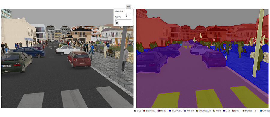
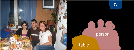
Semantic segmentation is a deep learning algorithm assigning a label or category to every pixel in an image. This technique is employed to identify groups of pixels representing distinct categories. For instance, in autonomous vehicles, semantic segmentation is crucial for recognizing vehicles, pedestrians, traffic signs, pavement, and other road features.
Semantic segmentation is a natural step in the progression from coarse to fine inference:The origin could be located at classification, which consists of making a prediction for a whole input.The next step is localization / detection, which provide not only the classes but also additional information regarding the spatial location of those classes.Finally, semantic segmentation achieves fine-grained inference by making dense predictions inferring labels for every pixel, so that each pixel is labeled with the class of its enclosing object ore region.
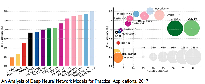
It is also worthy to review some standard deep networks that have made significant contributions to the field of computer vision, as they are often used as the basis of semantic segmentation systems:
- AlexNet: Toronto’s pioneering deep CNN that won the 2012 ImageNet competition with a test accuracy of 84.6%. It consists of 5 convolutional layers, max-pooling ones, ReLUs as non-linearities, 3 fully-convolutional layers, and dropout.
- VGG-16: This Oxford’s model won the 2013 ImageNet competition with 92.7% accuracy. It uses a stack of convolution layers with small receptive fields in the first layers instead of few layers with big receptive fields.
- GoogLeNet: This Google’s network won the 2014 ImageNet competition with accuracy of 93.3%. It is composed by 22 layers and a newly introduced building block called inception module. The module consists of a Network-in-Network layer, a pooling operation, a large-sized convolution layer, and small-sized convolution layer.
- ResNet: This Microsoft’s model won the 2016 ImageNet competition with 96.4 % accuracy. It is well-known due to its depth (152 layers) and the introduction of residual blocks. The residual blocks address the problem of training a really deep architecture by introducing identity skip connections so that layers can copy their inputs to the next layer.
What are the existing Semantic Segmentation approaches?
A general semantic segmentation architecture can be broadly thought of as an encoder network followed by a decoder network:
- The encoder is usually is a pre-trained classification network like VGG/ResNet followed by a decoder network.
- The task of the decoder is to semantically project the discriminative features (lower resolution) learnt by the encoder onto the pixel space (higher resolution) to get a dense classification.
Unlike classification where the end result of the very deep network is the only important thing, semantic segmentation not only requires discrimination at pixel level but also a mechanism to project the discriminative features learnt at different stages of the encoder onto the pixel space. Different approaches employ different mechanisms as a part of the decoding mechanism. Let’s explore the 3 main approaches:
1 — Region-Based Semantic Segmentation
The region-based methods generally follow the “segmentation using recognition” pipeline, which first extracts free-form regions from an image and describes them, followed by region-based classification. At test time, the region-based predictions are transformed to pixel predictions, usually by labeling a pixel according to the highest scoring region that contains it.
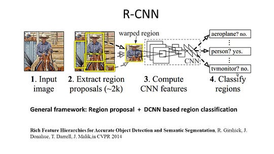
R-CNN (Regions with CNN feature) is one representative work for the region-based methods. It performs the semantic segmentation based on the object detection results. To be specific, R-CNN first utilizes selective search to extract a large quantity of object proposals and then computes CNN features for each of them. Finally, it classifies each region using the class-specific linear SVMs. Compared with traditional CNN structures which are mainly intended for image classification, R-CNN can address more complicated tasks, such as object detection and image segmentation, and it even becomes one important basis for both fields. Moreover, R-CNN can be built on top of any CNN benchmark structures, such as AlexNet, VGG, GoogLeNet, and ResNet.
For the image segmentation task, R-CNN extracted 2 types of features for each region: full region feature and foreground feature, and found that it could lead to better performance when concatenating them together as the region feature. R-CNN achieved significant performance improvements due to using the highly discriminative CNN features. However, it also suffers from a couple of drawbacks for the segmentation task:
- The feature is not compatible with the segmentation task.
- The feature does not contain enough spatial information for precise boundary generation.
- Generating segment-based proposals takes time and would greatly affect the final performance.
Due to these bottlenecks, recent research has been proposed to address the problems, including SDS, Hypercolumns, Mask R-CNN.
2 — Fully Convolutional Network-Based Semantic Segmentation
The original Fully Convolutional Network (FCN) learns a mapping from pixels to pixels, without extracting the region proposals. The FCN network pipeline is an extension of the classical CNN. The main idea is to make the classical CNN take as input arbitrary-sized images. The restriction of CNNs to accept and produce labels only for specific sized inputs comes from the fully-connected layers which are fixed. Contrary to them, FCNs only have convolutional and pooling layers which give them the ability to make predictions on arbitrary-sized inputs.
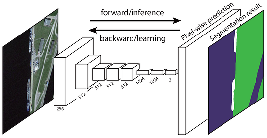
One issue in this specific FCN is that by propagating through several alternated convolutional and pooling layers, the resolution of the output feature maps is down sampled. Therefore, the direct predictions of FCN are typically in low resolution, resulting in relatively fuzzy object boundaries. A variety of more advanced FCN-based approaches have been proposed to address this issue, including SegNet, DeepLab-CRF, and Dilated Convolutions.
3 — Weakly Supervised Semantic Segmentation
Most of the relevant methods in semantic segmentation rely on a large number of images with pixel-wise segmentation masks. However, manually annotating these masks is quite time-consuming, frustrating and commercially expensive. Therefore, some weakly supervised methods have recently been proposed, which are dedicated to fulfilling the semantic segmentation by utilizing annotated bounding boxes.
For example, Boxsup employed the bounding box annotations as a supervision to train the network and iteratively improve the estimated masks for semantic segmentation. Simple Does It treated the weak supervision limitation as an issue of input label noise and explored recursive training as a de-noising strategy. Pixel-level Labeling interpreted the segmentation task within the multiple-instance learning framework and added an extra layer to constrain the model to assign more weight to important pixels for image-level classification.
Doing Semantic Segmentation with Fully-Convolutional Network
In this section, let’s walk through a step-by-step implementation of the most popular architecture for semantic segmentation — the Fully-Convolutional Net (FCN). We’ll implement it using the TensorFlow library in Python 3, along with other dependencies such as Numpy and Scipy.In this exercise we will label the pixels of a road in images using FCN. We’ll work with the Kitti Road Dataset for road/lane detection. This is a simple exercise from the Udacity’s Self-Driving Car Nano-degree program, which you can learn more about the setup in this GitHub repo.

Here are the key features of the FCN architecture:
- FCN transfers knowledge from VGG16 to perform semantic segmentation.
- The fully connected layers of VGG16 is converted to fully convolutional layers, using 1x1 convolution. This process produces a class presence heat map in low resolution.
- The upsampling of these low resolution semantic feature maps is done using transposed convolutions (initialized with bilinear interpolation filters).
- At each stage, the upsampling process is further refined by adding features from coarser but higher resolution feature maps from lower layers in VGG16.
- Skip connection is introduced after each convolution block to enable the subsequent block to extract more abstract, class-salient features from the previously pooled features.
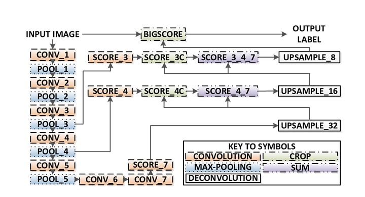
There are 3 versions of FCN (FCN-32, FCN-16, FCN-8). We’ll implement FCN-8, as detailed step-by-step below:
- Encoder: A pre-trained VGG16 is used as an encoder. The decoder starts from Layer 7 of VGG16.
- FCN Layer-8: The last fully connected layer of VGG16 is replaced by a 1x1 convolution.
- FCN Layer-9: FCN Layer-8 is upsampled 2 times to match dimensions with Layer 4 of VGG 16, using transposed convolution with parameters: (kernel=(4,4), stride=(2,2), paddding=’same’). After that, a skip connection was added between Layer 4 of VGG16 and FCN Layer-9.
- FCN Layer-10: FCN Layer-9 is upsampled 2 times to match dimensions with Layer 3 of VGG16, using transposed convolution with parameters: (kernel=(4,4), stride=(2,2), paddding=’same’). After that, a skip connection was added between Layer 3 of VGG 16 and FCN Layer-10.
- FCN Layer-11: FCN Layer-10 is upsampled 4 times to match dimensions with input image size so we get the actual image back and depth is equal to number of classes, using transposed convolution with parameters:(kernel=(16,16), stride=(8,8), paddding=’same’).
Step 1
We first load the pre-trained VGG-16 model into TensorFlow. Taking in the TensorFlow session and the path to the VGG Folder (which is downloadable here), we return the tuple of tensors from VGG model, including the image input, keep_prob (to control dropout rate), layer 3, layer 4, and layer 7.
def load_vgg(sess, vgg_path):

  # load the model and weights
  model = tf.saved_model.loader.load(sess, ['vgg16'], vgg_path)

  # Get Tensors to be returned from graph
  graph = tf.get_default_graph()
  image_input = graph.get_tensor_by_name('image_input:0')
  keep_prob = graph.get_tensor_by_name('keep_prob:0')
  layer3 = graph.get_tensor_by_name('layer3_out:0')
  layer4 = graph.get_tensor_by_name('layer4_out:0')
  layer7 = graph.get_tensor_by_name('layer7_out:0')

  return image_input, keep_prob, layer3, layer4, layer7
VGG16 function
Step 2
Now we focus on creating the layers for a FCN, using the tensors from the VGG model. Given the tensors for VGG layer output and the number of classes to classify, we return the tensor for the last layer of that output. In particular, we apply a 1x1 convolution to the encoder layers, and then add decoder layers to the network with skip connections and upsampling.
def layers(vgg_layer3_out, vgg_layer4_out, vgg_layer7_out, num_classes):

    # Use a shorter variable name for simplicity
    layer3, layer4, layer7 = vgg_layer3_out, vgg_layer4_out, vgg_layer7_out

    # Apply 1x1 convolution in place of fully connected layer
    fcn8 = tf.layers.conv2d(layer7, filters=num_classes, kernel_size=1, name="fcn8")

    # Upsample fcn8 with size depth=(4096?) to match size of layer 4 so that we can add skip connection with 4th layer
    fcn9 = tf.layers.conv2d_transpose(fcn8, filters=layer4.get_shape().as_list()[-1],
    kernel_size=4, strides=(2, 2), padding='SAME', name="fcn9")

    # Add a skip connection between current final layer fcn8 and 4th layer
    fcn9_skip_connected = tf.add(fcn9, layer4, name="fcn9_plus_vgg_layer4")

    # Upsample again
    fcn10 = tf.layers.conv2d_transpose(fcn9_skip_connected, filters=layer3.get_shape().as_list()[-1],
    kernel_size=4, strides=(2, 2), padding='SAME', name="fcn10_conv2d")

    # Add skip connection
    fcn10_skip_connected = tf.add(fcn10, layer3, name="fcn10_plus_vgg_layer3")

    # Upsample again
    fcn11 = tf.layers.conv2d_transpose(fcn10_skip_connected, filters=num_classes,
    kernel_size=16, strides=(8, 8), padding='SAME', name="fcn11")

    return fcn11
Layers function
Step 3
The next step is to optimize our neural network, aka building TensorFlow loss functions and optimizer operations. Here we use cross entropy as our loss function and Adam as our optimization algorithm.
def optimize(nn_last_layer, correct_label, learning_rate, num_classes):

  # Reshape 4D tensors to 2D, each row represents a pixel, each column a class
  logits = tf.reshape(nn_last_layer, (-1, num_classes), name="fcn_logits")
  correct_label_reshaped = tf.reshape(correct_label, (-1, num_classes))

  # Calculate distance from actual labels using cross entropy
  cross_entropy = tf.nn.softmax_cross_entropy_with_logits(logits=logits, labels=correct_label_reshaped[:])
  # Take mean for total loss
  loss_op = tf.reduce_mean(cross_entropy, name="fcn_loss")

  # The model implements this operation to find the weights/parameters that would yield correct pixel labels
  train_op = tf.train.AdamOptimizer(learning_rate=learning_rate).minimize(loss_op, name="fcn_train_op")

  return logits, train_op, loss_op
Optimize function
Step 4
Here we define the train_nn function, which takes in important parameters including number of epochs, batch size, loss function, optimizer operation, and placeholders for input images, label images, learning rate. For the training process, we also set keep_probability to 0.5 and learning_rate to 0.001. To keep track of the progress, we also print out the loss during training.
def train_nn(sess, epochs, batch_size, get_batches_fn, train_op,
             cross_entropy_loss, input_image,
             correct_label, keep_prob, learning_rate):

  keep_prob_value = 0.5
  learning_rate_value = 0.001
  for epoch in range(epochs):
      # Create function to get batches
      total_loss = 0
      for X_batch, gt_batch in get_batches_fn(batch_size):

          loss, _ = sess.run([cross_entropy_loss, train_op],
          feed_dict={input_image: X_batch, correct_label: gt_batch,
          keep_prob: keep_prob_value, learning_rate:learning_rate_value})

          total_loss += loss;

      print("EPOCH {} ...".format(epoch + 1))
      print("Loss = {:.3f}".format(total_loss))
      print()
Step 5
Finally, it’s time to train our net! In this run function, we first build our net using the load_vgg, layers, and optimize function. Then we train the net using the train_nn function and save the inference data for records.
def run():

  # Download pretrained vgg model
  helper.maybe_download_pretrained_vgg(data_dir)

  # A function to get batches
  get_batches_fn = helper.gen_batch_function(training_dir, image_shape)

  with tf.Session() as session:

    # Returns the three layers, keep probability and input layer from the vgg architecture
    image_input, keep_prob, layer3, layer4, layer7 = load_vgg(session, vgg_path)

    # The resulting network architecture from adding a decoder on top of the given vgg model
    model_output = layers(layer3, layer4, layer7, num_classes)

    # Returns the output logits, training operation and cost operation to be used
    # - logits: each row represents a pixel, each column a class
    # - train_op: function used to get the right parameters to the model to correctly label the pixels
    # - cross_entropy_loss: function outputting the cost which we are minimizing, lower cost should yield higher accuracy
    logits, train_op, cross_entropy_loss = optimize(model_output, correct_label, learning_rate, num_classes)

    # Initialize all variables
    session.run(tf.global_variables_initializer())
    session.run(tf.local_variables_initializer())

    print("Model build successful, starting training")

    # Train the neural network
    train_nn(session, EPOCHS, BATCH_SIZE, get_batches_fn,
             train_op, cross_entropy_loss, image_input,
             correct_label, keep_prob, learning_rate)

    # Run the model with the test images and save each painted output image (roads painted green)
    helper.save_inference_samples(runs_dir, data_dir, session, image_shape, logits, keep_prob, image_input)
Run function
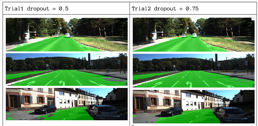
About our parameters, we choose epochs = 40, batch_size = 16, num_classes = 2, and image_shape = (160, 576). After doing 2 trial passes with dropout = 0.5 and dropout = 0.75, we found that the 2nd trial yields better results with better average losses.
To see the full code, check out this link: https://gist.github.com/khanhnamle1994/e2ff59ddca93c0205ac4e566d40b5e88
If you enjoyed this piece, I’d love it share it 👏 and spread the knowledge.


