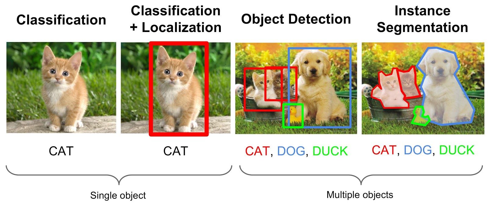
Deep learning has been very successful when working with images as data and is currently at a stage where it works better than humans on multiple use-cases. The most important problems that humans have been interested in solving with computer vision are image classification, object detection and segmentation in the increasing order of their difficulty.
In the plain old task of image classification we are just interested in getting the labels of all the objects that are present in an image. In object detection we come further a step and try to know along with what all objects that are present in an image, the location at which the objects are present with the help of bounding boxes. Image segmentation takes it to a new level by trying to find out accurately the exact boundary of the objects in the image.
In this article we will go through this concept of image segmentation, discuss the relevant use-cases, different neural network architectures involved in achieving the results, metrics and datasets to explore.
What is image segmentation
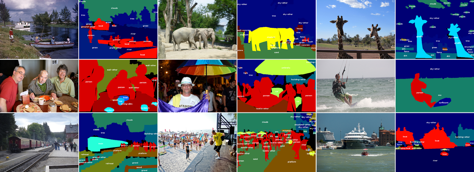
We know an image is nothing but a collection of pixels. Image segmentation is the process of classifying each pixel in an image belonging to a certain class and hence can be thought of as a classification problem per pixel. There are two types of segmentation techniques
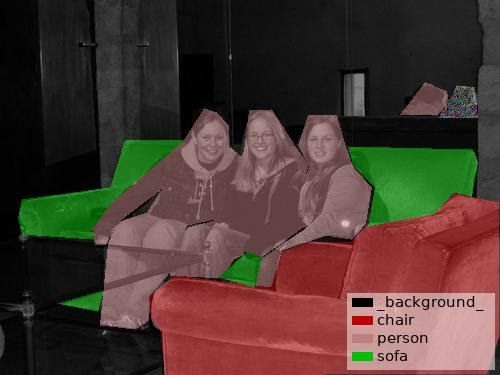
- Semantic segmentation: Semantic segmentation is the process of classifying each pixel belonging to a particular label. It doesn't different across different instances of the same object. For example if there are 2 cats in an image, semantic segmentation gives same label to all the pixels of both cats
- Instance segmentation: Instance segmentation differs from semantic segmentation in the sense that it gives a unique label to every instance of a particular object in the image. As can be seen in the image above all 3 dogs are assigned different colours i.e different labels. With semantic segmentation all of them would have been assigned the same colour.
So we will now come to the point where would we need this kind of an algorithm
Use-cases of image segmentation
1. Handwriting Recognition: Junjo et all demonstrated how semantic segmentation is being used to extract words and lines from handwritten documents in their 2019 research paper to recognise handwritten characters
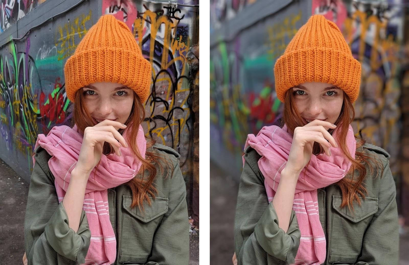
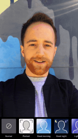
2. Google portrait mode: There are many use-cases where it is absolutely essential to separate foreground from background. For example in Google's portrait mode we can see the background blurred out while the foreground remains unchanged to give a cool effect
3. YouTube stories: Google recently released a feature YouTube stories for content creators to show different backgrounds while creating stories.
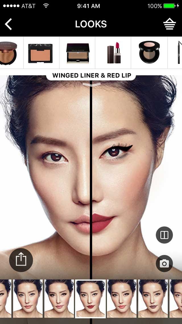
4. Virtual make-up: Applying virtual lip-stick is possible now with the help of image segmentation
5. Virtual try-on: Virtual try on of clothes is an interesting feature which was available in stores using specialized hardware which creates a 3d model. But with deep learning and image segmentation the same can be obtained using just a 2d image
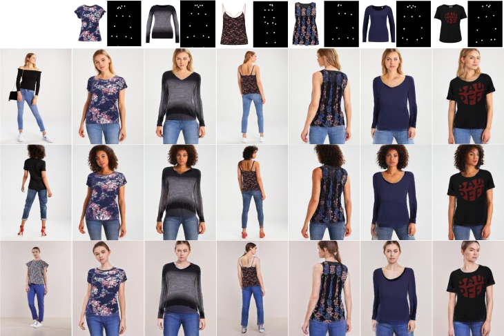
6. Visual Image Search: The idea of segmenting out clothes is also used in image retrieval algorithms in eCommerce. For example Pinterest/Amazon allows you to upload any picture and get related similar looking products by doing an image search based on segmenting out the cloth portion
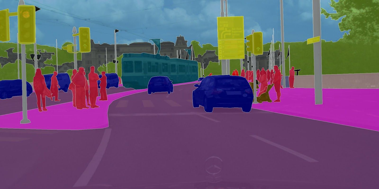
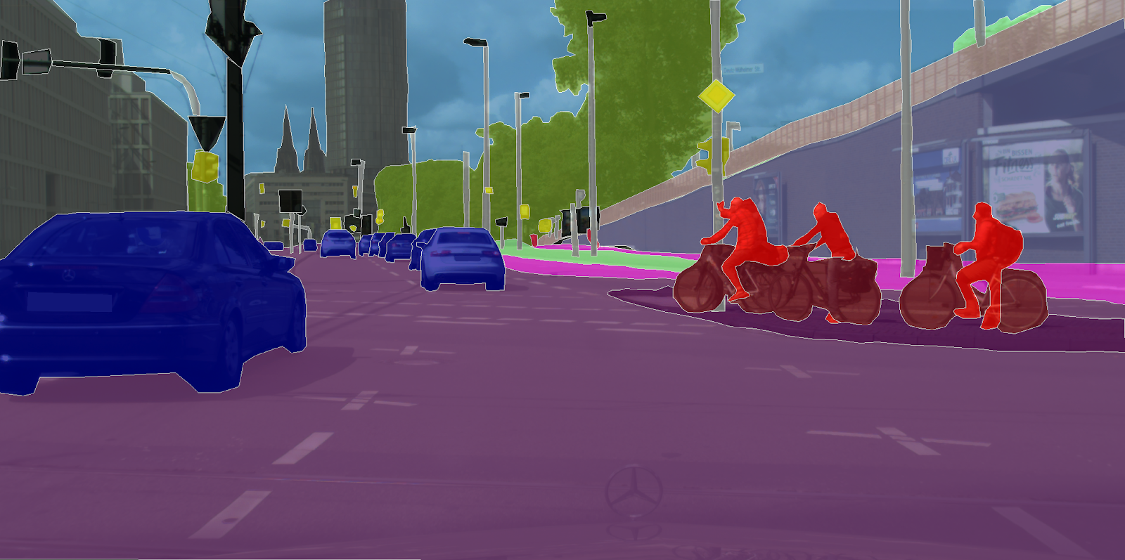
7. Self-driving cars: Self driving cars need a complete understanding of their surroundings to a pixel perfect level. Hence image segmentation is used to identify lanes and other necessary information
Methods and Techniques
Before the advent of deep learning, classical machine learning techniques like SVM, Random Forest, K-means Clustering were used to solve the problem of image segmentation. But as with most of the image related problem statements deep learning has worked comprehensively better than the existing techniques and has become a norm now when dealing with Semantic Segmentation. Let's review the techniques which are being used to solve the problem
Fully Convolutional Network
The general architecture of a CNN consists of few convolutional and pooling layers followed by few fully connected layers at the end. The paper of Fully Convolutional Network released in 2014 argues that the final fully connected layer can be thought of as doing a 1x1 convolution that cover the entire region.
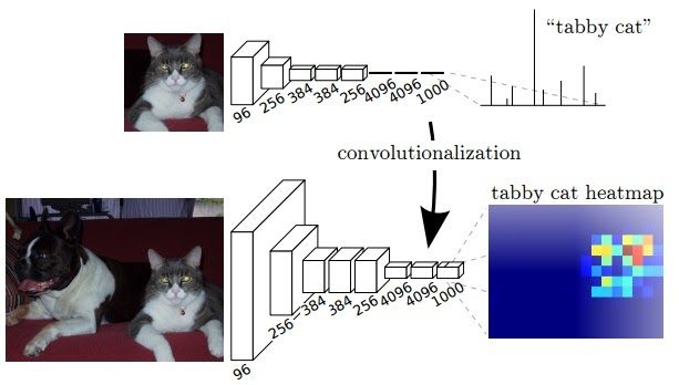
Hence the final dense layers can be replaced by a convolution layer achieving the same result. But now the advantage of doing this is the size of input need not be fixed anymore. When involving dense layers the size of input is constrained and hence when a different sized input has to be provided it has to be resized. But by replacing a dense layer with convolution, this constraint doesn't exist.
Also when a bigger size of image is provided as input the output produced will be a feature map and not just a class output like for a normal input sized image. Also the observed behavior of the final feature map represents the heatmap of the required class i.e the position of the object is highlighted in the feature map. Since the output of the feature map is a heatmap of the required object it is valid information for our use-case of segmentation.
Since the feature map obtained at the output layer is a down sampled due to the set of convolutions performed, we would want to up-sample it using an interpolation technique. Bilinear up sampling works but the paper proposes using learned up sampling with deconvolution which can even learn a non-linear up sampling.
The down sampling part of the network is called an encoder and the up sampling part is called a decoder. This is a pattern we will see in many architectures i.e reducing the size with encoder and then up sampling with decoder. In an ideal world we would not want to down sample using pooling and keep the same size throughout but that would lead to a huge amount of parameters and would be computationally infeasible.
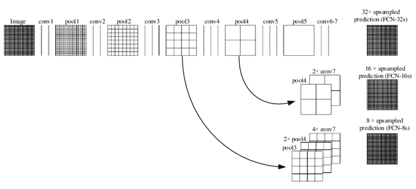
Although the output results obtained have been decent the output observed is rough and not smooth. The reason for this is loss of information at the final feature layer due to downsampling by 32 times using convolution layers. Now it becomes very difficult for the network to do 32x upsampling by using this little information. This architecture is called FCN-32
To address this issue, the paper proposed 2 other architectures FCN-16, FCN-8. In FCN-16 information from the previous pooling layer is used along with the final feature map and hence now the task of the network is to learn 16x up sampling which is better compared to FCN-32. FCN-8 tries to make it even better by including information from one more previous pooling layer.
Unet
U-net builds on top of the fully convolutional network from above. It was built for medical purposes to find tumours in lungs or the brain. It also consists of an encoder which down-samples the input image to a feature map and the decoder which up samples the feature map to input image size using learned deconvolution layers.
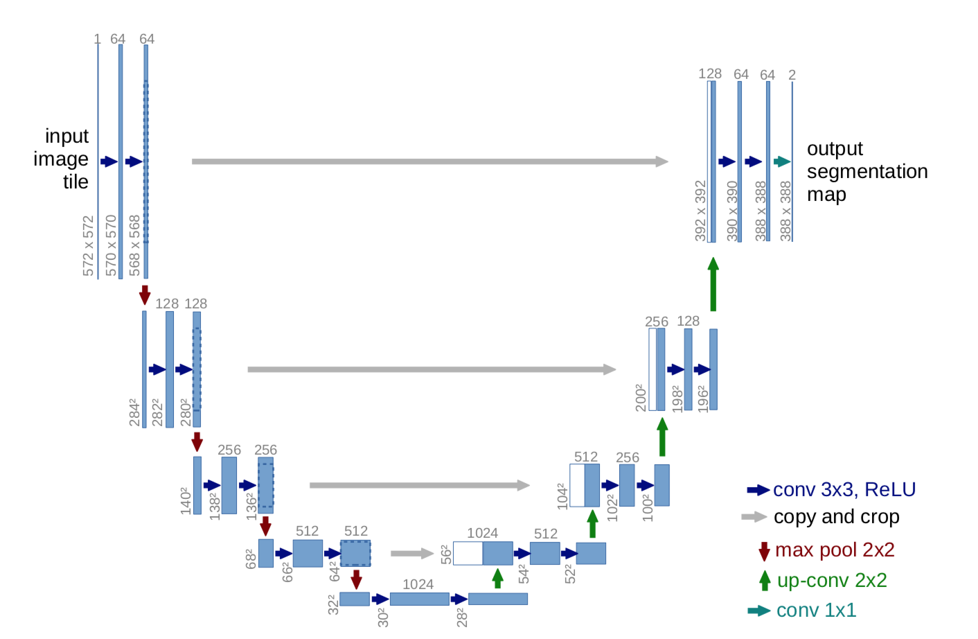
The main contribution of the U-Net architecture is the shortcut connections. We saw above in FCN that since we down-sample an image as part of the encoder we lost a lot of information which can't be easily recovered in the encoder part. FCN tries to address this by taking information from pooling layers before the final feature layer.
U-Net proposes a new approach to solve this information loss problem. It proposes to send information to every up sampling layer in decoder from the corresponding down sampling layer in the encoder as can be seen in the figure above thus capturing finer information whilst also keeping the computation low. Since the layers at the beginning of the encoder would have more information they would bolster the up sampling operation of decoder by providing fine details corresponding to the input images thus improving the results a lot. The paper also suggested use of a novel loss function which we will discuss below.
DeepLab
Deeplab from a group of researchers from Google have proposed a multitude of techniques to improve the existing results and get finer output at lower computational costs. The 3 main improvements suggested as part of the research are
1) Atrous convolutions
2) Atrous Spatial Pyramidal Pooling
3) Conditional Random Fields usage for improving final output
Let's discuss about all these
Atrous Convolution
One of the major problems with FCN approach is the excessive downsizing due to consecutive pooling operations. Due to series of pooling the input image is down sampled by 32x which is again up sampled to get the segmentation result. Downsampling by 32x results in a loss of information which is very crucial for getting fine output in a segmentation task. Also deconvolution to up sample by 32x is a computation and memory expensive operation since there are additional parameters involved in forming a learned up sampling.
The paper proposes the usage of Atrous convolution or the hole convolution or dilated convolution which helps in getting an understanding of large context using the same number of parameters.
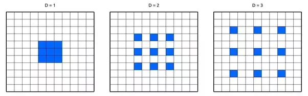
Dilated convolution works by increasing the size of the filter by appending zeros(called holes) to fill the gap between parameters. The number of holes/zeroes filled in between the filter parameters is called by a term dilation rate. When the rate is equal to 1 it is nothing but the normal convolution. When rate is equal to 2 one zero is inserted between every other parameter making the filter look like a 5x5 convolution. Now it has the capacity to get the context of 5x5 convolution while having 3x3 convolution parameters. Similarly for rate 3 the receptive field goes to 7x7.
In Deeplab last pooling layers are replaced to have stride 1 instead of 2 thereby keeping the down sampling rate to only 8x. Then a series of atrous convolutions are applied to capture the larger context. For training the output labelled mask is down sampled by 8x to compare each pixel. For inference, bilinear up sampling is used to produce output of the same size which gives decent enough results at lower computational/memory costs since bilinear up sampling doesn't need any parameters as opposed to deconvolution for up sampling.
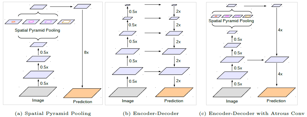
ASPP
Spatial Pyramidal Pooling is a concept introduced in SPPNet to capture multi-scale information from a feature map. Before the introduction of SPP input images at different resolutions are supplied and the computed feature maps are used together to get the multi-scale information but this takes more computation and time. With Spatial Pyramidal Pooling multi-scale information can be captured with a single input image.
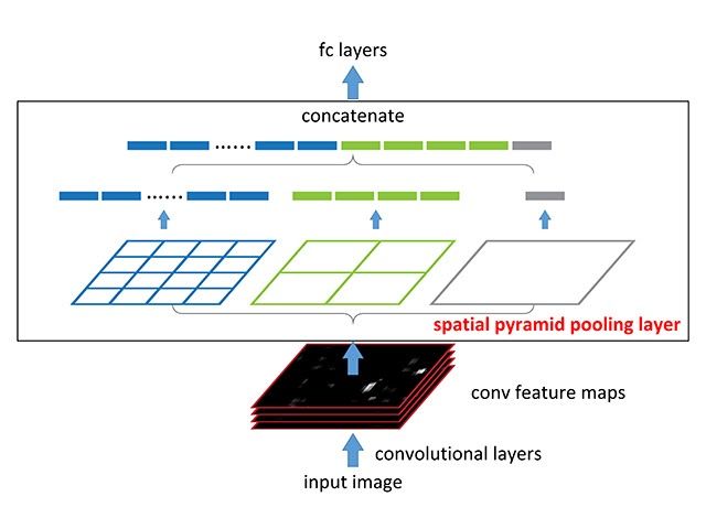
With the SPP module the network produces 3 outputs of dimensions 1x1(i.e GAP), 2x2 and 4x4. These values are concatenated by converting to a 1d vector thus capturing information at multiple scales. Another advantage of using SPP is input images of any size can be provided.
ASPP takes the concept of fusing information from different scales and applies it to Atrous convolutions. The input is convolved with different dilation rates and the outputs of these are fused together.
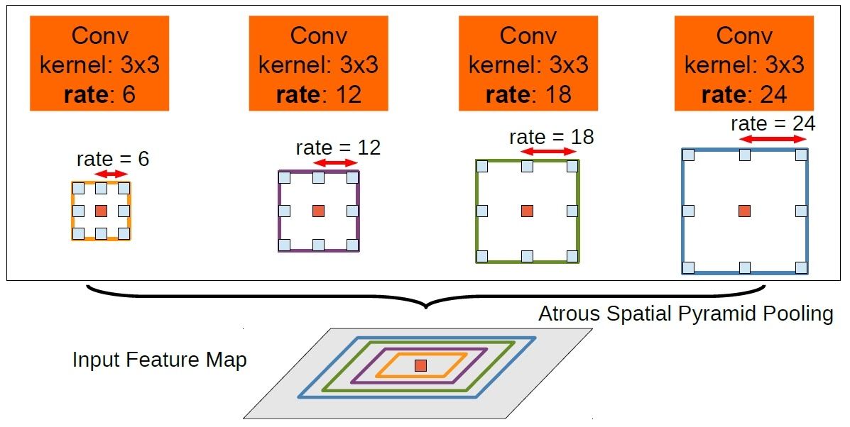
As can be seen the input is convolved with 3x3 filters of dilation rates 6, 12, 18 and 24 and the outputs are concatenated together since they are of same size. A 1x1 convolution output is also added to the fused output. To also provide the global information, the GAP output is also added to above after up sampling. The fused output of 3x3 varied dilated outputs, 1x1 and GAP output is passed through 1x1 convolution to get to the required number of channels.
Since the required image to be segmented can be of any size in the input the multi-scale information from ASPP helps in improving the results.
Improving output with CRF
Pooling is an operation which helps in reducing the number of parameters in a neural network but it also brings a property of invariance along with it. Invariance is the quality of a neural network being unaffected by slight translations in input. Due to this property obtained with pooling the segmentation output obtained by a neural network is coarse and the boundaries are not concretely defined.
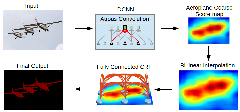
To deal with this the paper proposes use of graphical model CRF. Conditional Random Field operates a post-processing step and tries to improve the results produced to define shaper boundaries. It works by classifying a pixel based not only on it's label but also based on other pixel labels. As can be seen from the above figure the coarse boundary produced by the neural network gets more refined after passing through CRF.
Deeplab-v3 introduced batch normalization and suggested dilation rate multiplied by (1,2,4) inside each layer in a Resnet block. Also adding image level features to ASPP module which was discussed in the above discussion on ASPP was proposed as part of this paper
Deeplab-v3+ suggested to have a decoder instead of plain bilinear up sampling 16x. The decoder takes a hint from the decoder used by architectures like U-Net which take information from encoder layers to improve the results. The encoder output is up sampled 4x using bilinear up sampling and concatenated with the features from encoder which is again up sampled 4x after performing a 3x3 convolution. This approach yields better results than a direct 16x up sampling. Also modified Xception architecture is proposed to be used instead of Resnet as part of encoder and depthwise separable convolutions are now used on top of Atrous convolutions to reduce the number of computations.
Global Convolution Network
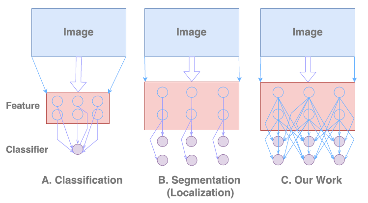
Semantic segmentation involves performing two tasks concurrently
i) Classification
ii) Localization
The classification networks are created to be invariant to translation and rotation thus giving no importance to location information whereas the localization involves getting accurate details w.r.t the location. Thus inherently these two tasks are contradictory. Most segmentation algorithms give more importance to localization i.e the second in the above figure and thus lose sight of global context. In this work the author proposes a way to give importance to classification task too while at the same time not losing the localization information
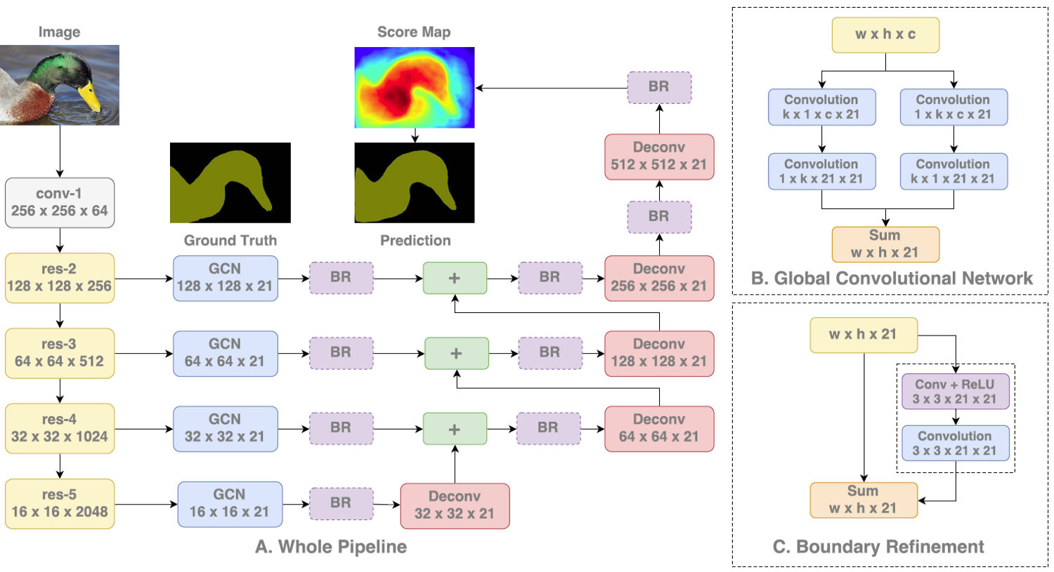
The author proposes to achieve this by using large kernels as part of the network thus enabling dense connections and hence more information. This is achieved with the help of a GCN block as can be seen in the above figure. GCN block can be thought of as a k x k convolution filter where k can be a number bigger than 3. To reduce the number of parameters a k x k filter is further split into 1 x k and k x 1, kx1 and 1xk blocks which are then summed up. Thus by increasing value k, larger context is captured.
In addition, the author proposes a Boundary Refinement block which is similar to a residual block seen in Resnet consisting of a shortcut connection and a residual connection which are summed up to get the result. It is observed that having a Boundary Refinement block resulted in improving the results at the boundary of segmentation.
Results showed that GCN block improved the classification accuracy of pixels closer to the center of object indicating the improvement caused due to capturing long range context whereas Boundary Refinement block helped in improving accuracy of pixels closer to boundary.
See More Than Once – KSAC for Semantic Segmentation
Deeplab family uses ASPP to have multiple receptive fields capture information using different atrous convolution rates. Although ASPP has been significantly useful in improving the segmentation of results there are some inherent problems caused due to the architecture. There is no information shared across the different parallel layers in ASPP thus affecting the generalization power of the kernels in each layer. Also since each layer caters to different sets of training samples(smaller objects to smaller atrous rate and bigger objects to bigger atrous rates), the amount of data for each parallel layer would be less thus affecting the overall generalizability. Also the number of parameters in the network increases linearly with the number of parameters and thus can lead to overfitting.
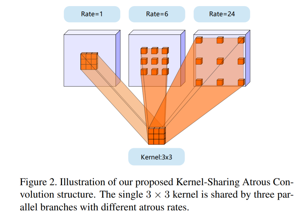
To handle all these issues the author proposes a novel network structure called Kernel-Sharing Atrous Convolution (KSAC). As can be seen in the above figure, instead of having a different kernel for each parallel layer is ASPP a single kernel is shared across thus improving the generalization capability of the network. By using KSAC instead of ASPP 62% of the parameters are saved when dilation rates of 6,12 and 18 are used.
Another advantage of using a KSAC structure is the number of parameters are independent of the number of dilation rates used. Thus we can add as many rates as possible without increasing the model size. ASPP gives best results with rates 6,12,18 but accuracy decreases with 6,12,18,24 indicating possible overfitting. But KSAC accuracy still improves considerably indicating the enhanced generalization capability.
This kernel sharing technique can also be seen as an augmentation in the feature space since the same kernel is applied over multiple rates. Similar to how input augmentation gives better results, feature augmentation performed in the network should help improve the representation capability of the network.
Video Segmentation
For use cases like self-driving cars, robotics etc. there is a need for real-time segmentation on the observed video. The architectures discussed so far are pretty much designed for accuracy and not for speed. So if they are applied on a per-frame basis on a video the result would come at very low speed.
Also generally in a video there is a lot of overlap in scenes across consecutive frames which could be used for improving the results and speed which won't come into picture if analysis is done on a per-frame basis. Using these cues let's discuss architectures which are specifically designed for videos
STFCN
Spatio-Temporal FCN proposes to use FCN along with LSTM to do video segmentation. We are already aware of how FCN can be used to extract features for segmenting an image. LSTM are a kind of neural networks which can capture sequential information over time. STFCN combines the power of FCN with LSTM to capture both the spatial information and temporal information
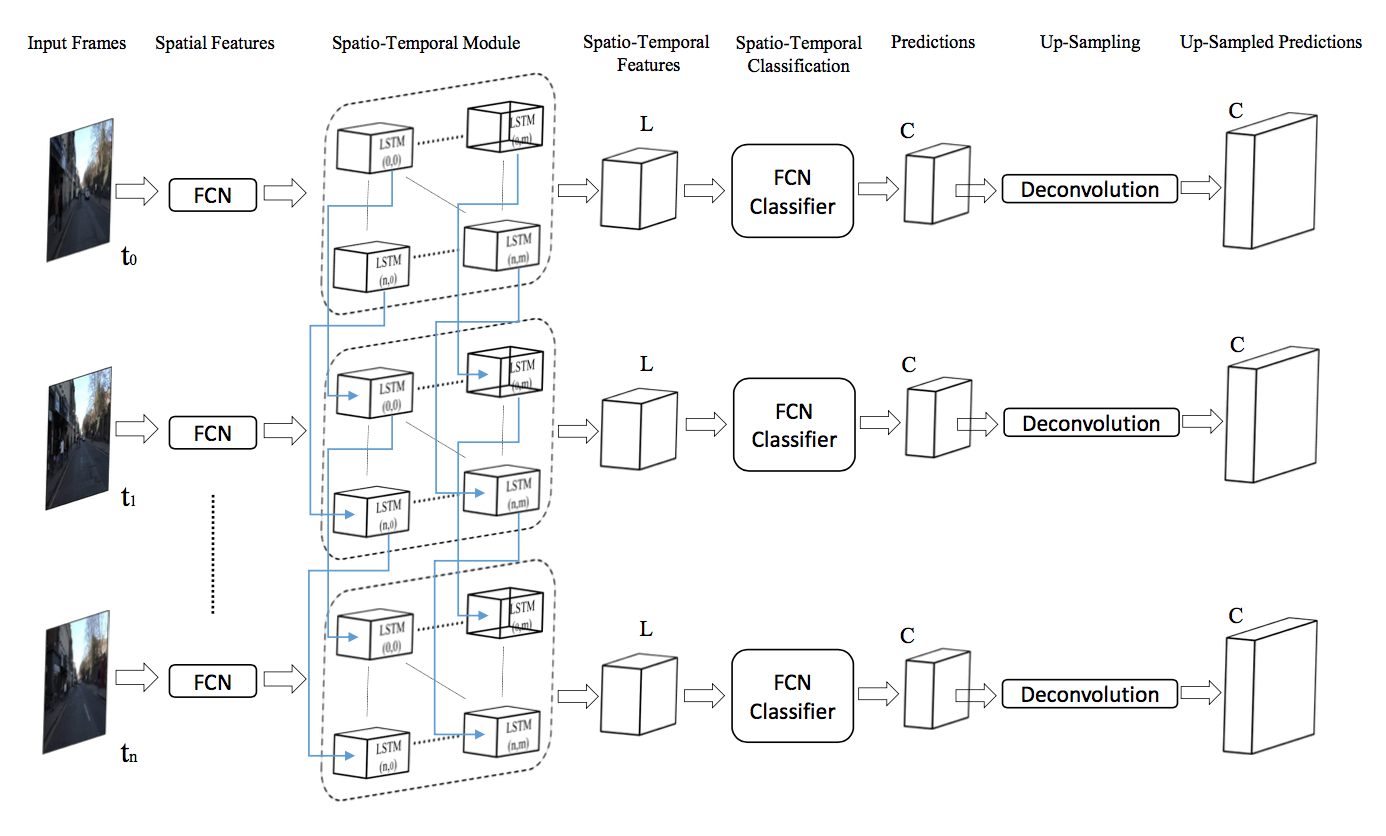
As can be seen from the above figure STFCN consists of a FCN, Spatio-temporal module followed by deconvolution. The feature map produced by a FCN is sent to Spatio-Temporal Module which also has an input from the previous frame's module. The module based on both these inputs captures the temporal information in addition to the spatial information and sends it across which is up sampled to the original size of image using deconvolution similar to how it's done in FCN
Since both FCN and LSTM are working together as part of STFCN the network is end to end trainable and outperforms single frame segmentation approaches. There are similar approaches where LSTM is replaced by GRU but the concept is same of capturing both the spatial and temporal information
Semantic Video CNNs through Representation Warping
This paper proposes the use of optical flow across adjacent frames as an extra input to improve the segmentation results
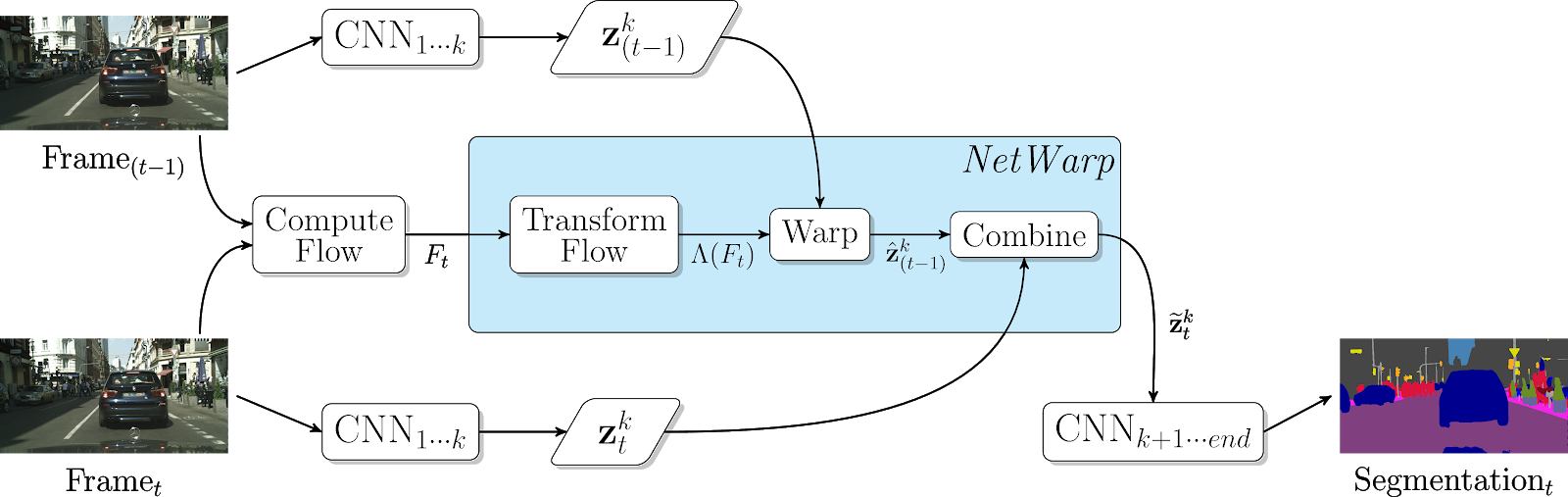
The approach suggested can be roped in to any standard architecture as a plug-in. The key ingredient that is at play is the NetWarp module. To compute the segmentation map the optical flow between the current frame and previous frame is calculated i.e Ft and is passed through a FlowCNN to get Λ(Ft) . This process is called Flow Transformation. This value is passed through a warp module which also takes as input the feature map of an intermediate layer calculated by passing through the network. This gives a warped feature map which is then combined with the intermediate feature map of the current layer and the entire network is end to end trained. This architecture achieved SOTA results on CamVid and Cityscapes video benchmark datasets.
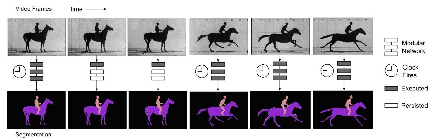
Clockwork Convnets for Video Semantic Segmentation
This paper proposes to improve the speed of execution of a neural network for segmentation task on videos by taking advantage of the fact that semantic information in a video changes slowly compared to pixel level information. So the information in the final layers changes at a much slower pace compared to the beginning layers. The paper suggests different times
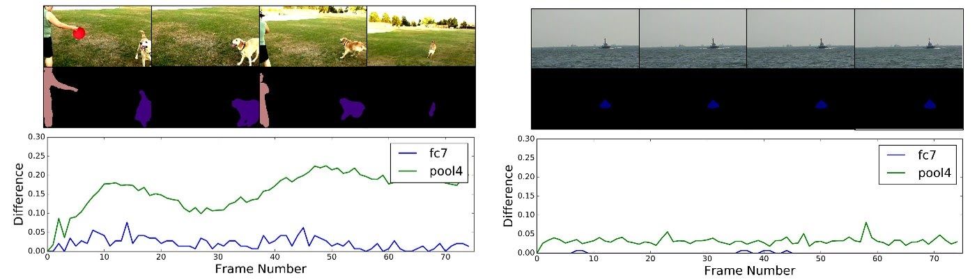
The above figure represents the rate of change comparison for a mid level layer pool4 and a deep layer fc7. On the left we see that since there is a lot of change across the frames both the layers show a change but the change for pool4 is higher. In the right we see that there is not a lot of change across the frames. Hence pool4 shows marginal change whereas fc7 shows almost nil change.
The research utilizes this concept and suggests that in cases where there is not much of a change across the frames there is no need of computing the features/outputs again and the cached values from the previous frame can be used. Since the rate of change varies with layers different clocks can be set for different sets of layers. When the clock ticks the new outputs are calculated, otherwise the cached results are used. The rate of clock ticks can be statically fixed or can be dynamically learnt
Low-Latency Video Semantic Segmentation
This paper improves on top of the above discussion by adaptively selecting the frames to compute the segmentation map or to use the cached result instead of using a fixed timer or a heuristic.
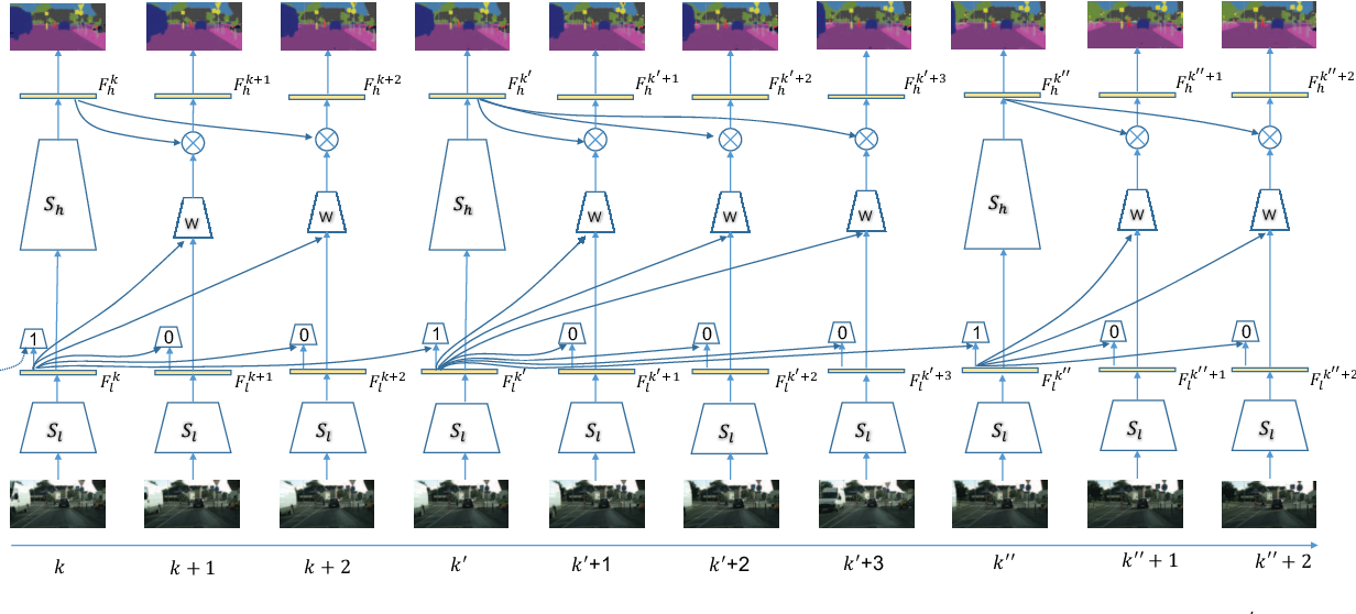
The paper proposes to divide the network into 2 parts, low level features and high level features. The cost of computing low level features in a network is much less compared to higher features. The research suggests to use the low level network features as an indicator of the change in segmentation map. In their observations they found strong correlation between low level features change and the segmentation map change. So to understand if there is a need to compute if the higher features are needed to be calculated, the lower features difference across 2 frames is found and is compared if it crosses a particular threshold. This entire process is automated by a small neural network whose task is to take lower features of two frames and to give a prediction as to whether higher features should be computed or not. Since the network decision is based on the input frames the decision taken is dynamic compared to the above approach.
Segmentation for point clouds
Data coming from a sensor such as lidar is stored in a format called Point Cloud. Point cloud is nothing but a collection of unordered set of 3d data points(or any dimension). It is a sparse representation of the scene in 3d and CNN can't be directly applied in such a case. Also any architecture designed to deal with point clouds should take into consideration that it is an unordered set and hence can have a lot of possible permutations. So the network should be permutation invariant. Also the points defined in the point cloud can be described by the distance between them. So closer points in general carry useful information which is useful for segmentation tasks
PointNet
PointNet is an important paper in the history of research on point clouds using deep learning to solve the tasks of classification and segmentation. Let's study the architecture of Pointnet
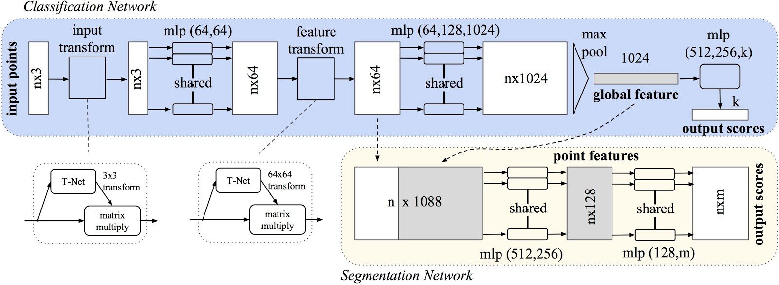
Input of the network for n points is an n x 3 matrix. n x 3 matrix is mapped to n x 64 using a shared multi-perceptron layer(fully connected network) which is then mapped to n x 64 and then to n x 128 and n x 1024. Max pooling is applied to get a 1024 vector which is converted to k outputs by passing through MLP's with sizes 512, 256 and k. Finally k class outputs are produced similar to any classification network.
Classification deals only with the global features but segmentation needs local features as well. So the local features from intermediate layer at n x 64 is concatenated with global features to get a n x 1088 matrix which is sent through mlp of 512 and 256 to get to n x 256 and then though MLP's of 128 and m to give m output classes for every point in point cloud.
Also the network involves an input transform and feature transform as part of the network whose task is to not change the shape of input but add invariance to affine transformations i.e translation, rotation etc.
A-CNN
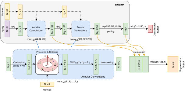
A-CNN proposes the usage of Annular convolutions to capture spatial information. We know from CNN that convolution operations capture the local information which is essential to get an understanding of the image. A-CNN devised a new convolution called Annular convolution which is applied to neighbourhood points in a point-cloud.
The architecture takes as input n x 3 points and finds normals for them which is used for ordering of points. A subsample of points is taken using the FPS algorithm resulting in ni x 3 points. On these annular convolution is applied to increase to 128 dimensions. Annular convolution is performed on the neighbourhood points which are determined using a KNN algorithm.
Another set of the above operations are performed to increase the dimensions to 256. Then an mlp is applied to change the dimensions to 1024 and pooling is applied to get a 1024 global vector similar to point-cloud. This entire part is considered the encoder. For classification the encoder global output is passed through mlp to get c class outputs. For segmentation task both the global and local features are considered similar to PointCNN and is then passed through an MLP to get m class outputs for each point.
Metrics
Let's discuss the metrics which are generally used to understand and evaluate the results of a model.
Pixel Accuracy
Pixel accuracy is the most basic metric which can be used to validate the results. Accuracy is obtained by taking the ratio of correctly classified pixels w.r.t total pixels
Accuracy = (TP+TN)/(TP+TN+FP+FN)
The main disadvantage of using such a technique is the result might look good if one class overpowers the other. Say for example the background class covers 90% of the input image we can get an accuracy of 90% by just classifying every pixel as background
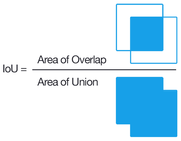
Intersection Over Union
IOU is defined as the ratio of intersection of ground truth and predicted segmentation outputs over their union. If we are calculating for multiple classes, IOU of each class is calculated and their mean is taken. It is a better metric compared to pixel accuracy as if every pixel is given as background in a 2 class input the IOU value is (90/100+0/100)/2 i.e 45% IOU which gives a better representation as compared to 90% accuracy.
Frequency weighted IOU
This is an extension over mean IOU which we discussed and is used to combat class imbalance. If one class dominates most part of the images in a dataset like for example background, it needs to be weighed down compared to other classes. Thus instead of taking the mean of all the class results, a weighted mean is taken based on the frequency of the class region in the dataset.
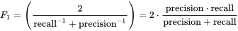
F1 Score
The metric popularly used in classification F1 Score can be used for segmentation task as well to deal with class imbalance.
Average Precision
Area under the Precision - Recall curve for a chosen threshold IOU average over different classes is used for validating the results.
Loss functions
Loss function is used to guide the neural network towards optimization. Let's discuss a few popular loss functions for semantic segmentation task.
Cross Entropy Loss
Simple average of cross-entropy classification loss for every pixel in the image can be used as an overall function. But this again suffers due to class imbalance which FCN proposes to rectify using class weights
UNet tries to improve on this by giving more weight-age to the pixels near the border which are part of the boundary as compared to inner pixels as this makes the network focus more on identifying borders and not give a coarse output.
Focal Loss
Focal loss was designed to make the network focus on hard examples by giving more weight-age and also to deal with extreme class imbalance observed in single-stage object detectors. The same can be applied in semantic segmentation tasks as well
Dice Loss
Dice function is nothing but F1 score. This loss function directly tries to optimize F1 score. Similarly direct IOU score can be used to run optimization as well
Tversky Loss
It is a variant of Dice loss which gives different weight-age to FN and FP
Hausdorff distance
It is a technique used to measure similarity between boundaries of ground truth and predicted. It is calculated by finding out the max distance from any point in one boundary to the closest point in the other. Reducing directly the boundary loss function is a recent trend and has been shown to give better results especially in use-cases like medical image segmentation where identifying the exact boundary plays a key role.
The advantage of using a boundary loss as compared to a region based loss like IOU or Dice Loss is it is unaffected by class imbalance since the entire region is not considered for optimization, only the boundary is considered.

The two terms considered here are for two boundaries i.e the ground truth and the output prediction.
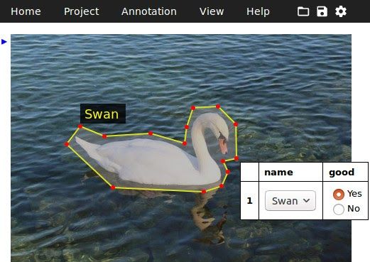
Annotation tools
1. LabelMe:
Image annotation tool written in python.
Supports polygon annotation.
Open Source and free.
Runs on Windows, Mac, Ubuntu or via Anaconda, Docker
Link
2. Computer Vision Annotation Tool:
Video and image annotation tool developed by Intel
Free and available online
Runs on Windows, Mac and Ubuntu
Link
3. Vgg image annotator:
Free open source image annotation tool
Simple html page < 200kb and can run offline
Supports polygon annotation and points.
Link
4. Rectlabel:
Paid annotation tool for Mac
Can use core ML models to pre-annotate the images
Supports polygons, cubic-bezier, lines, and points
Link
6. Labelbox:
Paid annotation tool
Supports pen tool for faster and accurate annotation
Link
Datasets
As part of this section let's discuss various popular and diverse datasets available in the public which one can use to get started with training.
Pascal Context:
This dataset is an extension of Pascal VOC 2010 dataset and goes beyond the original dataset by providing annotations for the whole scene and has 400+ classes of real-world data.
COCO Dataset:
The COCO stuff dataset has 164k images of the original COCO dataset with pixel level annotations and is a common benchmark dataset. It covers 172 classes: 80 thing classes, 91 stuff classes and 1 class 'unlabeled'
Cityscapes Dataset:
This dataset consists of segmentation ground truths for roads, lanes, vehicles and objects on road. The dataset contains 30 classes and of 50 cities collected over different environmental and weather conditions. Has also a video dataset of finely annotated images which can be used for video segmentation. KITTI and CamVid are similar kinds of datasets which can be used for training self-driving cars.
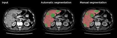
Lits Dataset:
The dataset was created as part of a challenge to identify tumor lesions from liver CT scans. The dataset contains 130 CT scans of training data and 70 CT scans of testing data.
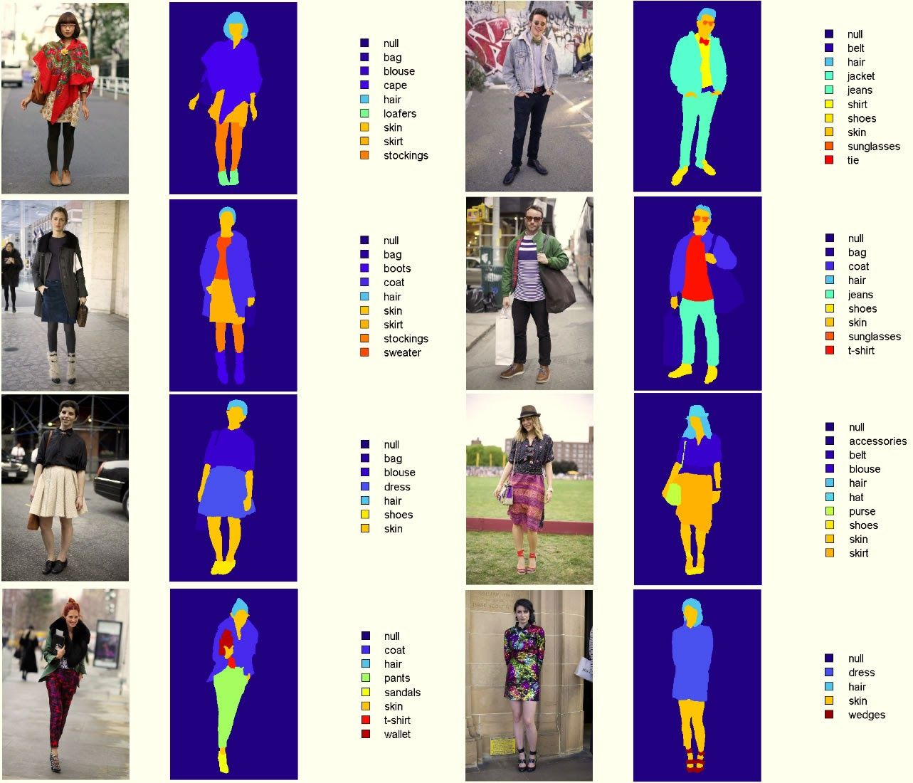
CCP Dataset:
Cloth Co-Parsing is a dataset which is created as part of research paper Clothing Co-Parsing by Joint Image Segmentation and Labeling . The dataset contains 1000+ images with pixel level annotations for a total of 59 tags.
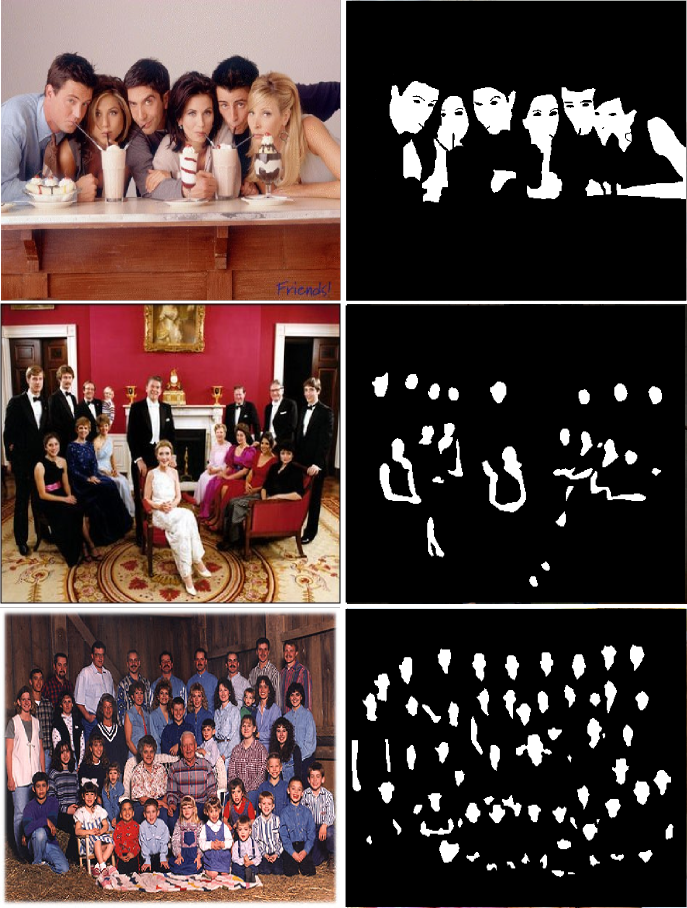
Pratheepan Dataset:
A dataset created for the task of skin segmentation based on images from google containing 32 face photos and 46 family photos
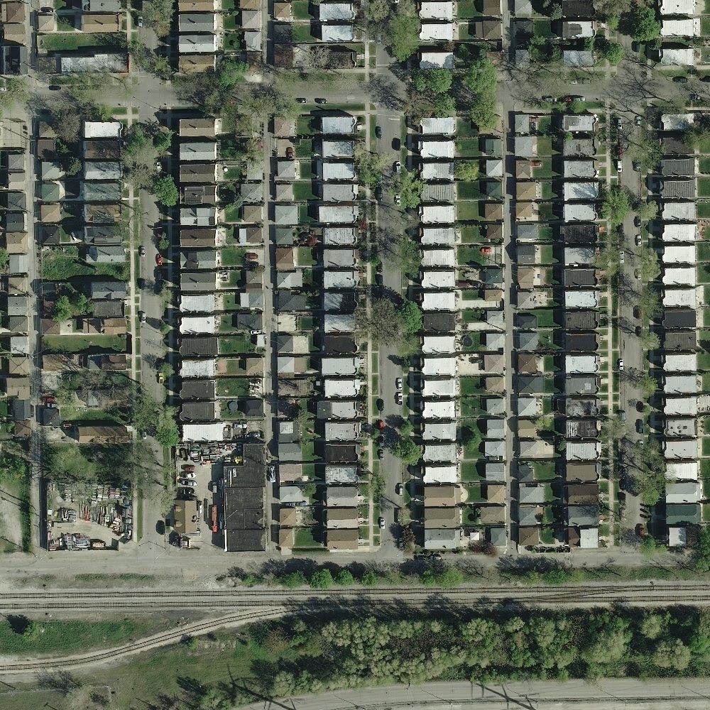
Inria Aerial Image Labeling:
A dataset of aerial segmentation maps created from public domain images. Has a coverage of 810 sq km and has 2 classes building and not-building.
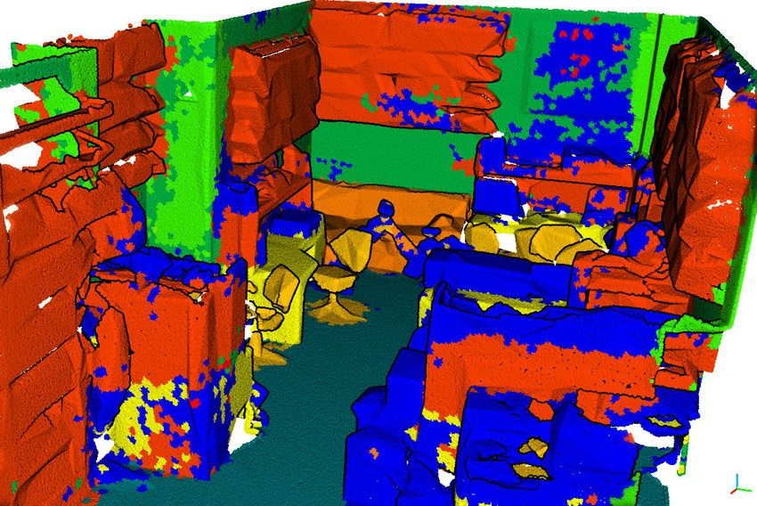
S3DIS:
This dataset contains the point clouds of six large scale indoor parts in 3 buildings with over 70000 images.
Summary
We have discussed a taxonomy of different algorithms which can be used for solving the use-case of semantic segmentation be it on images, videos or point-clouds and also their contributions and limitations. We also looked through the ways to evaluate the results and the datasets to get started on. This should give a comprehensive understanding on semantic segmentation as a topic in general.
To get a list of more resources for semantic segmentation, check out this resource